Unconstrained Model Predictive Control
Unconstrained Model Predictive Control (MPC) provides a foundation for understanding the core principles of predictive control without the complexity of constraint handling. This document presents the complete mathematical derivation and implementation of unconstrained MPC for linear systems.
Problem Formulation
System Model
Consider a discrete-time linear time-invariant system:
Where:
- : state vector at time step
- : control input vector at time step
- : state transition matrix
- : input matrix
Performance Function
The finite-horizon cost function is:
Where:
- : prediction horizon (number of future steps to consider)
- : terminal weight matrix ()
- : state weight matrix ()
- : input weight matrix ()
- : Positive semi-definite (allow regulation to zero)
- : Positive definite (ensures unique solution)
- These matrices determine the relative importance of different objectives
Prediction Horizon Formulation
State Predictions
At time step , the future states are predicted as:
Compact Matrix Notation
For efficient computation, define the stacked vectors:
Predicted state vector:
Control input vector:
Matrix Form of Predictions
The prediction equation becomes:
Where:
Prediction matrix for states:
Prediction matrix for inputs:
- Each row block of contains representing the effect of initial state after steps
- Each element of contains representing the effect of input on state
Quadratic Programming Transformation
Objective: Standard QP Form
To solve the MPC problem efficiently, we transform it into standard quadratic programming form:
Step 1: Separate Initial State Cost
Rewrite the cost function by extracting the initial state term:
Step 2: Define Block Diagonal Matrices
State weight matrix for prediction horizon:
Input weight matrix for prediction horizon:
Step 3: Express Cost in Matrix Form
The cost function becomes:
Step 4: Substitute Prediction Equation
Substituting :
Expanding:
Step 5: Final QP Form
Collecting terms:
Where:
Hessian matrix:
Linear term coefficient:
Constant term:
The constant term depends only on the current state and doesn't affect the optimization. We can ignore it when solving for the optimal control sequence.
Analytical Solution
Unconstrained Optimization
For the unconstrained case, the optimal control sequence is found by setting the gradient to zero:
Optimal control sequence:
Extracting the First Control
Since MPC applies only the first control action:
This gives us the MPC feedback law:
Where the MPC feedback gain is:
Implementation
MATLAB Implementation
QP Transformation Function
function [Ap, Bp, Qp, Rp, F, H] = QP_Transform(A, B, Q, R, Qf, Np)
%% QP_Transform - Transform MPC cost function into standard QP form
%
% This function transforms the MPC cost function into standard QP form
% for efficient numerical solution.
%
% Inputs:
%   A, B - System matrices
%   Q, R, Qf - Weight matrices
%   Np - Prediction horizon
%
% Outputs:
%   Ap, Bp - Prediction matrices
%   Qp, Rp - Block diagonal weight matrices
%   F, H - QP problem matrices

n = size(A, 1);  % Number of states
p = size(B, 2);  % Number of inputs

% Initialize prediction matrices
Ap = zeros(Np*n, n);
Bp = zeros(Np*n, Np*p);

% Build prediction matrix Ap = [A; A^2; ...; A^Np]
for i = 1:Np
    Ap((i-1)*n+1:i*n, :) = A^i;
end

% Build prediction matrix Bp
for i = 1:Np
    for j = 1:i
        Bp((i-1)*n+1:i*n, (j-1)*p+1:j*p) = A^(i-j) * B;
    end
end

% Build block diagonal weight matrices
% Qp = diag(Q, Q, ..., Q, Qf)
Qp = kron(eye(Np-1), Q);
Qp = blkdiag(Qp, Qf);

% Rp = diag(R, R, ..., R)
Rp = kron(eye(Np), R);

% Compute QP matrices
F = Bp' * Qp * Ap;       % Linear term coefficient
H = Bp' * Qp * Bp + Rp;  % Hessian matrix

end
MPC vs LQR Comparison
%% MPC vs LQR Comparison
%----------------------------------------------------------%
% Compare performance of unconstrained MPC and LQR
%----------------------------------------------------------%
clear; close all; clc;
set(0, 'DefaultAxesFontName', 'Times New Roman')
set(0, 'DefaultAxesFontSize', 14)

%% System Model
A = [0 1; 0.5 0];
n = size(A, 1);
B = [0; 1];
p = size(B, 2);

% Simulation parameters
Time = 3;        % Total simulation time
ts = 0.1;        % Sampling time
k_steps = Time/ts;  % Number of simulation steps

%% Weight Matrices
Q = [1 0; 0 1];   % State weight matrix
Qf = [1 0; 0 1];  % Terminal weight matrix
R = 1;            % Input weight matrix

%% Initialization
Np = 5;                    % Prediction horizon
x0 = [10; 5];             % Initial state
x_lqr = x0;               % LQR state
x_mpc = x0;               % MPC state

% History arrays
xh_lqr = zeros(n, k_steps+1);
xh_mpc = zeros(n, k_steps+1);
uh_lqr = zeros(p, k_steps);
uh_mpc = zeros(p, k_steps);

xh_lqr(:, 1) = x_lqr;
xh_mpc(:, 1) = x_mpc;

%% Controller Design
% LQR gain
K_lqr = lqr(A, B, Q, R);

% MPC matrices
[Ap, Bp, Qp, Rp, F, H] = QP_Transform(A, B, Q, R, Qf, Np);

%% Simulation Loop
for k = 1:k_steps
    %% MPC Control
    % Solve QP problem: min 0.5*U'*H*U + (F*x_mpc)'*U
    options = optimoptions('quadprog', 'Display', 'off');
    U_opt = quadprog(H, F*x_mpc, [], [], [], [], [], [], [], options);
    u_mpc = U_opt(1:p);  % Extract first control action

    % Update MPC system
    x_mpc = A * x_mpc + B * u_mpc;

    % Store results
    xh_mpc(:, k+1) = x_mpc;
    uh_mpc(:, k) = u_mpc;

    %% LQR Control
    u_lqr = -K_lqr * x_lqr;

    % Update LQR system
    x_lqr = A * x_lqr + B * u_lqr;

    % Store results
    xh_lqr(:, k+1) = x_lqr;
    uh_lqr(:, k) = u_lqr;
end

%% Plotting
figure('Position', [100, 100, 800, 600]);

% State x1
subplot(3, 1, 1);
plot(0:k_steps, xh_lqr(1, :), 'b-', 'LineWidth', 2);
hold on;
plot(0:k_steps, xh_mpc(1, :), 'r--', 'LineWidth', 2);
legend('LQR', 'MPC', 'FontSize', 12);
xlabel('Time step');
ylabel('State x_1');
title('State x_1 Response');
grid on;

% State x2
subplot(3, 1, 2);
plot(0:k_steps, xh_lqr(2, :), 'b-', 'LineWidth', 2);
hold on;
plot(0:k_steps, xh_mpc(2, :), 'r--', 'LineWidth', 2);
legend('LQR', 'MPC', 'FontSize', 12);
xlabel('Time step');
ylabel('State x_2');
title('State x_2 Response');
grid on;

% Control input
subplot(3, 1, 3);
plot(0:k_steps-1, uh_lqr(1, :), 'b-', 'LineWidth', 2);
hold on;
plot(0:k_steps-1, uh_mpc(1, :), 'r--', 'LineWidth', 2);
legend('LQR', 'MPC', 'FontSize', 12);
xlabel('Time step');
ylabel('Control Input u');
title('Control Effort');
grid on;

sgtitle('MPC vs LQR Performance Comparison', 'FontSize', 16, 'FontWeight', 'bold');
Python Implementation
import numpy as np
import matplotlib.pyplot as plt
from scipy.optimize import minimize
from scipy.linalg import solve_discrete_are

def qp_transform(A, B, Q, R, Qf, Np):
    """Transform MPC cost function into standard QP form"""
    n, p = A.shape[0], B.shape[1]

    # Build prediction matrix Ap
    Ap = np.zeros((Np*n, n))
    A_power = np.eye(n)
    for i in range(Np):
        A_power = A_power @ A
        Ap[i*n:(i+1)*n, :] = A_power

    # Build prediction matrix Bp
    Bp = np.zeros((Np*n, Np*p))
    for i in range(Np):
        for j in range(i+1):
            Bp[i*n:(i+1)*n, j*p:(j+1)*p] = np.linalg.matrix_power(A, i-j) @ B

    # Build block diagonal weight matrices
    Qp = np.kron(np.eye(Np-1), Q)
    Qp = np.block([[Qp, np.zeros((Qp.shape[0], Qf.shape[1]))],
                   [np.zeros((Qf.shape[0], Qp.shape[1])), Qf]])

    Rp = np.kron(np.eye(Np), R)

    # Compute QP matrices
    F = Bp.T @ Qp @ Ap
    H = Bp.T @ Qp @ Bp + Rp

    return Ap, Bp, Qp, Rp, F, H

def mpc_unconstrained(A, B, Q, R, Qf, x0, k_steps, Np):
    """Unconstrained MPC simulation"""
    n, p = A.shape[0], B.shape[1]

    # Get QP matrices
    _, _, _, _, F, H = qp_transform(A, B, Q, R, Qf, Np)

    # Initialize arrays
    x_traj = np.zeros((n, k_steps+1))
    u_traj = np.zeros((p, k_steps))
    x_traj[:, 0] = x0

    x = x0.copy()

    for k in range(k_steps):
        # Solve QP problem: min 0.5*U'*H*U + (F*x)'*U
        def objective(U):
            return 0.5 * U.T @ H @ U + (F @ x).T @ U

        # Initial guess
        U0 = np.zeros(Np * p)

        # Solve optimization
        result = minimize(objective, U0, method='BFGS')
        U_opt = result.x

        # Extract first control action
        u = U_opt[:p]
        u_traj[:, k] = u

        # Update state
        x = A @ x + B @ u
        x_traj[:, k+1] = x

    return x_traj, u_traj

# System matrices
A = np.array([[0, 1], [0.5, 0]])
B = np.array([[0], [1]])

# Weight matrices
Q = np.eye(2)
Qf = np.eye(2)
R = np.array([[1]])

# Simulation parameters
x0 = np.array([10, 5])
k_steps = 30
Np = 5

# MPC simulation
x_mpc, u_mpc = mpc_unconstrained(A, B, Q, R, Qf, x0, k_steps, Np)

# LQR for comparison
P = solve_discrete_are(A, B, Q, R)
K_lqr = np.linalg.solve(R + B.T @ P @ B, B.T @ P @ A)

# LQR simulation
x_lqr = np.zeros((2, k_steps+1))
u_lqr = np.zeros((1, k_steps))
x_lqr[:, 0] = x0

x = x0.copy()
for k in range(k_steps):
    u = -K_lqr @ x
    u_lqr[:, k] = u
    x = A @ x + B @ u
    x_lqr[:, k+1] = x

# Plotting
fig, (ax1, ax2, ax3) = plt.subplots(3, 1, figsize=(10, 8))

# State x1
ax1.plot(range(k_steps+1), x_lqr[0, :], 'b-', linewidth=2, label='LQR')
ax1.plot(range(k_steps+1), x_mpc[0, :], 'r--', linewidth=2, label='MPC')
ax1.set_ylabel('State $x_1$')
ax1.set_title('State $x_1$ Response')
ax1.legend()
ax1.grid(True)

# State x2
ax2.plot(range(k_steps+1), x_lqr[1, :], 'b-', linewidth=2, label='LQR')
ax2.plot(range(k_steps+1), x_mpc[1, :], 'r--', linewidth=2, label='MPC')
ax2.set_ylabel('State $x_2$')
ax2.set_title('State $x_2$ Response')
ax2.legend()
ax2.grid(True)

# Control input
ax3.plot(range(k_steps), u_lqr[0, :], 'b-', linewidth=2, label='LQR')
ax3.plot(range(k_steps), u_mpc[0, :], 'r--', linewidth=2, label='MPC')
ax3.set_xlabel('Time step')
ax3.set_ylabel('Control Input $u$')
ax3.set_title('Control Effort')
ax3.legend()
ax3.grid(True)

plt.tight_layout()
plt.suptitle('MPC vs LQR Performance Comparison', fontsize=16, fontweight='bold', y=0.98)
plt.show()
Analysis: MPC vs LQR
Performance Comparison
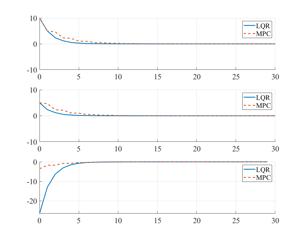
The simulation results demonstrate several key differences between unconstrained MPC and LQR:
Weight Matrix Effects
Case 1:
- High penalty on : Both controllers prioritize position regulation
- MPC shows similar performance to LQR but with slightly different transients
- Both achieve fast convergence of position state
Case 2:
- Balanced state penalties: Equal importance on both states
- MPC exhibits more conservative behavior initially
- Similar steady-state performance for both controllers
Case 3:
- High input penalty: Both controllers use minimal control effort
- Slower convergence but smoother control action
- MPC shows slightly different input profile due to finite horizon
Key Observations
-
Finite Horizon Effects:
- MPC considers only future steps, while LQR assumes infinite horizon
- This can lead to slightly different control strategies, especially early in the response
-
Terminal Cost Importance:
- The choice of affects MPC performance significantly
- Setting equal to the infinite-horizon LQR cost matrix often improves performance
-
Computational Differences:
- LQR: One-time gain computation, constant feedback law
- MPC: Online optimization at each time step, adaptive behavior
-
Equivalence Conditions:
- For very long prediction horizons, unconstrained MPC approaches LQR performance
- With proper terminal cost design, even short horizons can achieve good performance
Design Guidelines
Prediction Horizon Selection
Short horizons ():
- Fast computation
- May sacrifice performance
- Suitable for fast systems or limited computational resources
Medium horizons ():
- Good balance between performance and computation
- Covers most system dynamics
- Recommended for most applications
Long horizons ():
- Approaches infinite-horizon performance
- Higher computational cost
- May be unnecessary for many systems
Weight Matrix Tuning
State weights ():
- Reflect relative importance of different states
- should account for future behavior beyond horizon
- Consider setting as solution to infinite-horizon ARE
Input weights ():
- Balance performance vs. control effort
- Larger values → more conservative control
- Consider actuator limitations and energy constraints
Computational Considerations
Matrix conditioning:
- Ensure is well-conditioned for numerical stability
- Check eigenvalues of for positive definiteness
- Consider regularization if necessary
Efficient implementation:
- Pre-compute constant matrices (, ) when possible
- Use warm-starting for iterative solvers
- Exploit structure in QP problem for faster solution
Extensions and Future Topics
1. Constrained MPC
- Inequality constraints on states and inputs
- Constraint handling and feasibility
- Active set methods and interior-point algorithms
2. Robust MPC
- Model uncertainties and disturbances
- Tube-based MPC
- Min-max optimization
3. Nonlinear MPC
- Nonlinear system models
- Nonlinear programming solvers
- Successive linearization approaches
4. Economic MPC
- Economic objective functions
- Integration of control and optimization
- Performance vs. economics trade-offs
Summary
Unconstrained MPC provides:
- Systematic framework for finite-horizon optimal control
- Natural extension of LQR to finite horizons
- Foundation for understanding constrained MPC
- Computational efficiency through QP formulation
The analytical solution reveals the direct relationship between MPC and LQR, while the finite horizon introduces important design considerations for practical implementation.
References
- Rawlings, J. B., Mayne, D. Q., & Diehl, M. (2017). Model Predictive Control: Theory, Computation, and Design (2nd ed.). Nob Hill Publishing.
- Rakovic, S. V., & Levine, W. S. (2018). Handbook of Model Predictive Control. Birkhäuser.
- Wang, T. (2023). 控制之美 (卷2). Tsinghua University Press.
- Maciejowski, J. M. (2002). Predictive Control: With Constraints. Pearson Education.