Introduction to Model Predictive Control

Model Predictive Control (MPC), also known as Receding Horizon Control, is an advanced control strategy that solves an optimal control problem over a finite prediction horizon at each sampling time. This document provides a comprehensive introduction to MPC fundamentals and implementation.

MPC Overview

Core Concept

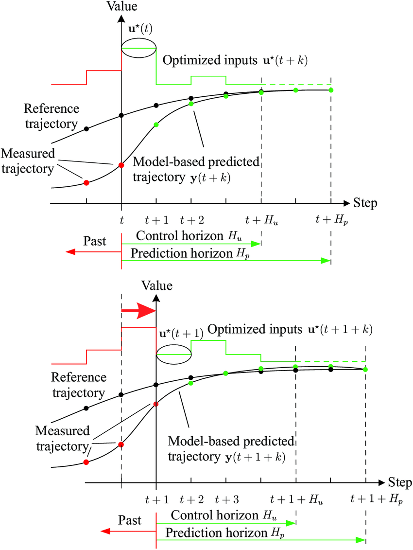
MPC is based on the principle of receding horizon optimization:

1. Predict future system behavior over a prediction horizon
2. Optimize control actions to minimize a cost function
3. Apply only the first optimal control action
4. Repeat the process at the next time step with updated measurements

This approach provides several advantages:

• Constraint handling: Natural incorporation of system constraints
• Multivariable control: Systematic handling of MIMO systems
• Preview capabilities: Ability to utilize future reference information
• Robustness: Online optimization adapts to disturbances and uncertainties

Why "Receding Horizon"?

The optimization horizon moves forward in time at each sampling instant, always maintaining the same horizon length. This creates a "receding" effect where the future optimization window slides forward continuously.

Mathematical Formulation

System Model

Consider a discrete-time nonlinear system: $x_{k+1} = f(x_k, u_k)$

Where:

• $x_k \in \mathbb{R}^n$: state vector at time $k$
• $u_k \in \mathbb{R}^p$: control input vector at time $k$
• $f(\cdot)$: system dynamics (potentially nonlinear)

Performance Function

The MPC optimization problem is formulated as: $J = h(x_N, x_d) + \sum_{k=1}^{N_p-1} g(x_k, x_d, u_k)$

Where:

• $N_p$: prediction horizon (number of future time steps to consider)
• $N_c$: control horizon (number of control moves to optimize)
• $x_d$: desired reference trajectory
• $h(\cdot)$: terminal cost function
• $g(\cdot)$: stage cost function

Horizon Relationship

Commonly, we set $N_p = N_c$ for simplicity, although different horizons can be used based on specific requirements:

• $N_p > N_c$: Control becomes constant after $N_c$ steps
• $N_p = N_c$: Full control authority over prediction horizon

MPC Algorithm Steps

At each time step $k$, MPC performs:

Step 1: State Measurement/Estimation

• Obtain current state $x_k$ (measured or estimated)

Step 2: Optimization

• Solve for optimal control sequence: $(u_{k|k}, u_{k+1|k}, \ldots, u_{k+N_c-1|k})$
• Predict future states: $(x_{k+1|k}, x_{k+2|k}, \ldots, x_{k+N_p|k})$

Step 3: Control Application

• Apply only the first control action: $u_k = u_{k|k}$

Step 4: Horizon Shift

• Move to time $k+1$ and repeat the process

Notation Convention

• $u_{k+i|k}$: Control action calculated at time $k$ to be applied at time $k+i$
• $x_{k+i|k}$: State predicted at time $k$ for time $k+i$
• $|$: Conditional notation indicating "given information at time"

Quadratic Programming Foundation

Why Quadratic Programming?

For linear systems with quadratic cost functions, MPC reduces to a Quadratic Programming (QP) problem, which can be solved efficiently using well-established numerical methods.

General QP Formulation

A quadratic program has the form:

Minimize: $J = \frac{1}{2}x^T Q x + R^T x$

Subject to:

$$\begin{aligned} Ax &\leq b &&\text{(inequality constraints)} \\ A_{eq}x &= b_{eq} &&\text{(equality constraints)} \\ x_L &\leq x \leq x_U &&\text{(bound constraints)} \end{aligned}$$

Where:

• $x \in \mathbb{R}^n$: optimization variables (control sequence in MPC)
• $Q \in \mathbb{R}^{n \times n}$: positive semi-definite Hessian matrix
• $R \in \mathbb{R}^n$: linear term vector
• $A, A_{eq}$: constraint matrices
• $b, b_{eq}$: constraint vectors
• $x_L, x_U$: variable bounds

Case A: Unconstrained Optimization

When there are no constraints and $Q$ is positive definite:

Optimality condition:

$$\frac{\partial J}{\partial x} = Qx + R = 0$$

Analytical solution:

$$x^* = -Q^{-1}R$$

Second-order condition:

$$\frac{\partial^2 J}{\partial x^2} = Q > 0 \quad \text{(ensures minimum)}$$

Case B: Equality Constraints

For problems with equality constraints $A_{eq}x = b_{eq}$, we use the Lagrange multiplier method.

Lagrangian function: $L = \frac{1}{2}x^T Q x + R^T x + \lambda^T(A_{eq}x - b_{eq})$

Optimality conditions: $\frac{\partial L}{\partial x} = Qx + R + A_{eq}^T\lambda = 0$ $\frac{\partial L}{\partial \lambda} = A_{eq}x - b_{eq} = 0$

System of equations: $\begin{bmatrix} Q & A_{eq}^T \\ A_{eq} & 0 \end{bmatrix} \begin{bmatrix} x \\ \lambda \end{bmatrix} = \begin{bmatrix} -R \\ b_{eq} \end{bmatrix}$

Solution (if inverse exists): $\begin{bmatrix} x^* \\ \lambda^* \end{bmatrix} = \begin{bmatrix} Q & A_{eq}^T \\ A_{eq} & 0 \end{bmatrix}^{-1} \begin{bmatrix} -R \\ b_{eq} \end{bmatrix}$

Case C: Inequality Constraints

For problems with inequality constraints, analytical solutions are generally not available. Numerical methods are required:

Common solution methods:

• Interior-point methods: Efficient for large problems
• Active-set methods: Good for small to medium problems
• Gradient-based methods: Simple but potentially slow convergence

Implementation Tools

MATLAB Implementation

MATLAB provides built-in optimization tools for QP problems:

% Quadratic programming solver
x = quadprog(Q, R, A, b, Aeq, beq, xL, xU);

% With options for algorithm selection
options = optimoptions('quadprog', 'Algorithm', 'interior-point');
x = quadprog(Q, R, A, b, Aeq, beq, xL, xU, [], options);

Key parameters:

• Q, R: Objective function matrices
• A, b: Inequality constraint matrices
• Aeq, beq: Equality constraint matrices
• xL, xU: Variable bounds

CasADi Framework

CasADi is an open-source tool for nonlinear optimization supporting multiple platforms:

Python example:

import casadi as ca

# Define optimization variables
x = ca.MX.sym('x', n)

# Define objective function
J = 0.5 * ca.mtimes([x.T, Q, x]) + ca.mtimes(R.T, x)

# Define constraints
g = []  # constraint expressions
lbg = []  # lower bounds
ubg = []  # upper bounds

# Create optimization problem
nlp = {'x': x, 'f': J, 'g': ca.vertcat(*g)}
solver = ca.nlpsol('solver', 'ipopt', nlp)

# Solve
sol = solver(x0=x_init, lbg=lbg, ubg=ubg, lbx=x_L, ubx=x_U)
x_opt = sol['x']

MATLAB example:

import casadi.*

% Define optimization variables
x = MX.sym('x', n);

% Define objective function
J = 0.5 * x' * Q * x + R' * x;

% Define constraints
g = [];  % Add constraints as needed

% Create optimization problem
nlp = struct('x', x, 'f', J, 'g', vertcat(g));
solver = nlpsol('solver', 'ipopt', nlp);

% Solve
sol = solver('x0', x_init, 'lbg', lbg, 'ubg', ubg, ...
            'lbx', x_L, 'ubx', x_U);
x_opt = full(sol.x);

MPC Design Considerations

1. Horizon Selection

Prediction horizon ($N_p$):

• Longer horizons: Better performance, higher computational cost
• Shorter horizons: Faster computation, potentially degraded performance
• Rule of thumb: Choose $N_p$ to cover system settling time

Control horizon ($N_c$):

• $N_c < N_p$: Reduced computational burden, control becomes constant
• $N_c = N_p$: Full control flexibility, higher computational cost

2. Cost Function Design

State penalties:

• Weight matrices $Q$ should reflect relative importance of states
• Larger weights → tighter regulation of corresponding states

Control penalties:

• Weight matrices $R$ balance control effort vs. performance
• Larger weights → more conservative control action

Terminal cost:

• Function $h(x_N, x_d)$ ensures stability for finite horizons
• Often chosen as infinite-horizon LQR cost

3. Constraint Formulation

Input constraints: $u_{\min} \leq u_k \leq u_{\max}$

State constraints: $x_{\min} \leq x_k \leq x_{\max}$

Slew rate constraints: $\Delta u_{\min} \leq u_k - u_{k-1} \leq \Delta u_{\max}$

Advantages and Limitations

Advantages

1. Natural constraint handling: Incorporates physical limitations directly
2. Multivariable capability: Systematic approach for MIMO systems
3. Predictive nature: Uses model to anticipate future behavior
4. Flexibility: Accommodates time-varying references and constraints
5. Online optimization: Adapts to disturbances and model uncertainties

Limitations

1. Computational requirements: Online optimization can be demanding
2. Model dependency: Performance relies on model accuracy
3. Parameter tuning: Requires careful selection of horizons and weights
4. Feasibility issues: Constraints may lead to infeasible problems
5. Stability guarantees: Require careful design for finite horizons

Applications

Industrial Applications

• Chemical processes: Refineries, petrochemical plants
• Power systems: Grid control, renewable energy integration
• Automotive: Engine control, autonomous driving
• Aerospace: Flight control, trajectory optimization
• Manufacturing: Robotics, process optimization

Academic Research Areas

• Robust MPC: Handling model uncertainties
• Stochastic MPC: Dealing with random disturbances
• Economic MPC: Optimizing economic objectives
• Distributed MPC: Large-scale system control
• Learning-based MPC: Integration with machine learning

Summary

Model Predictive Control represents a paradigm shift in control system design:

• From reactive to predictive: Uses model to anticipate future behavior
• From unconstrained to constrained: Natural incorporation of physical limitations
• From SISO to MIMO: Systematic handling of multivariable systems
• From fixed to adaptive: Online optimization enables real-time adaptation

The combination of prediction, optimization, and constraint handling makes MPC particularly suitable for complex, multivariable systems with operating constraints.

Next Steps

To fully understand MPC implementation:

1. Study unconstrained MPC: Linear systems with quadratic costs
2. Explore constraint handling: QP formulation and solution methods
3. Analyze stability: Terminal constraints and costs
4. Implement examples: Simple systems to understand behavior
5. Advanced topics: Robust MPC, nonlinear MPC, economic MPC

References

1. Rawlings, J. B., Mayne, D. Q., & Diehl, M. (2017). Model Predictive Control: Theory, Computation, and Design (2nd ed.). Nob Hill Publishing.
2. Rakovic, S. V., & Levine, W. S. (2018). Handbook of Model Predictive Control. Birkhäuser.
3. Camacho, E. F., & Alba, C. B. (2013). Model Predictive Control (2nd ed.). Springer-Verlag.
4. CH02-QuadraticProgramming.pdf (Berkeley)
5. What Is Model Predictive Control? - MATLAB
6. CasADi - A symbolic framework for automatic differentiation