Dynamic Programming and Bellman Optimality Principle

Dynamic programming provides a systematic approach to solving optimal control problems by decomposing complex problems into simpler subproblems. This document introduces the fundamental concepts and demonstrates the method through a practical drone control example.

Bellman Optimality Principle

The Bellman Optimality Principle states:

"An optimal policy has the property that whatever the initial state and initial decision are, the remaining decisions must constitute an optimal policy with regard to the state resulting from the first decision."

Key insights:

• Universal principle: Applies regardless of initial state and decision
• Optimal substructure: Remaining decisions must be optimal for the resulting state
• Foundation for dynamic programming: Enables backward recursive solution

Dynamic Programming Definition

Dynamic programming is a computational method that applies the Bellman optimality principle to solve optimal control problems efficiently by avoiding redundant calculations through systematic storage and reuse of subproblem solutions.

Problem Setup: Drone Vertical Movement

System Model

Consider a simple drone moving vertically with the following dynamics:

State-space representation:

$$\dot{x}(t) = \begin{bmatrix} 0 & 1 \\ 0 & 0 \end{bmatrix} x + \begin{bmatrix} 0 \\ 1 \end{bmatrix} u$$

State vector:

$$x(t) = \begin{bmatrix} x_1(t) \\ x_2(t) \end{bmatrix} = \begin{bmatrix} h(t) \\ v(t) \end{bmatrix}$$

Where:

• $h(t)$: position (height) of drone
• $v(t)$: velocity of drone

Problem Parameters

Initial state:

$$x_0 = \begin{bmatrix} 0 \\ 0 \end{bmatrix}$$

Target state:

$$x_d = \begin{bmatrix} 10 \\ 0 \end{bmatrix}$$

Constraints:

• Input constraint: $-3 \text{ m/s}^2 \leq u \leq 2 \text{ m/s}^2$
• Velocity constraint: $0 \text{ m/s} \leq x_2 \leq 3 \text{ m/s}$

Objective (minimum time):

$$J = \int_{t_0}^{t_f} dt = t_f - t_0$$

State Space Discretization

To apply dynamic programming, we discretize the continuous state space into a finite grid.

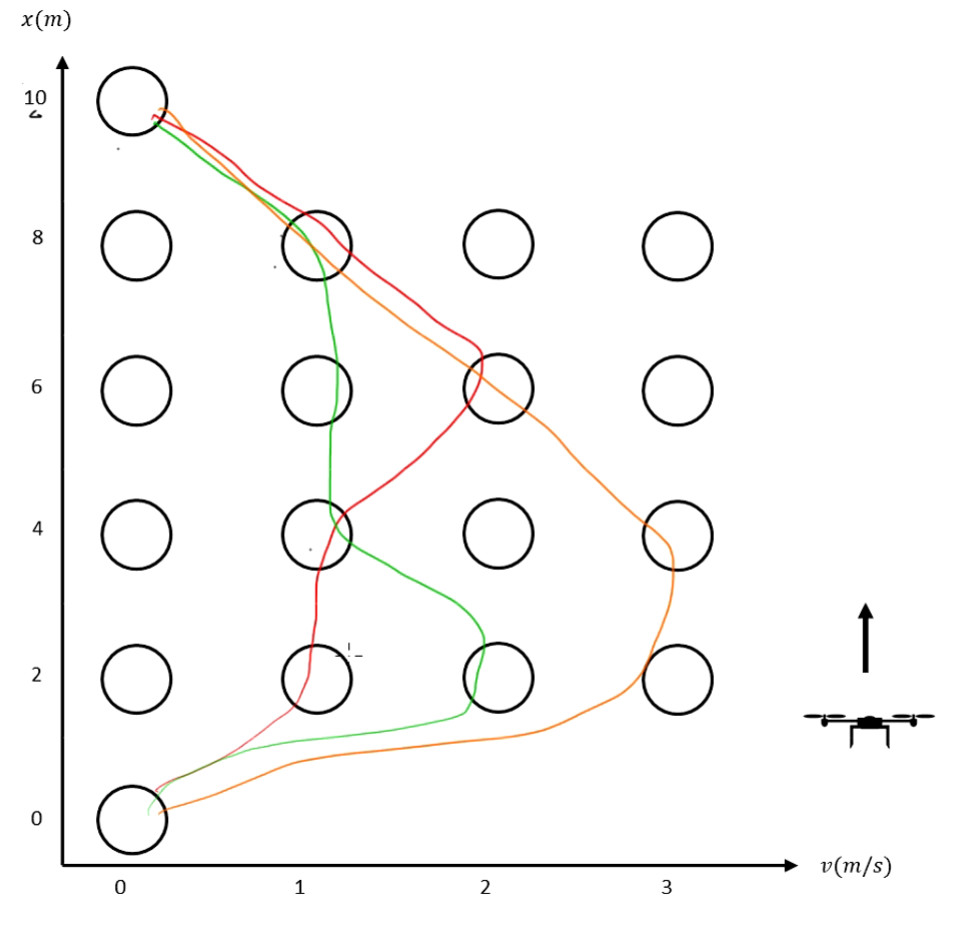
Discretization scheme:

• Height ($x_1$): 5 intervals → 6 nodes
• Velocity ($x_2$): 3 intervals → 4 nodes
• Total states: $6 \times 4 = 24$ nodes

Markov Property

The discretized system satisfies the Markov property: the future state depends only on the current state and action, not on the history of states.

Solution Approaches Comparison

Brute Force Search (Exhaustive Method)

Computational complexity:

$$\text{Number of paths} = n_{x_2}^{(n_{x_1}-2)} = 4^{(6-2)} = 256$$

Characteristics:

• ✅ Guarantees global optimum
• ❌ Exponential computational complexity
• ❌ Becomes intractable for large state spaces

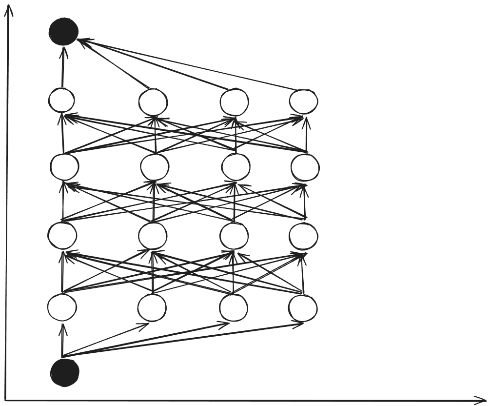
Dynamic Programming (Backward Multi-stage)

Computational complexity:

$$\text{Number of calculations} = (n_{x_1}-2) \cdot n_{x_2}^2 + 2 \cdot n_{x_2} = 4 \cdot 16 + 2 \cdot 4 = 72$$

Characteristics:

• ✅ Polynomial computational complexity
• ✅ Systematic and optimal
• ✅ Enables offline computation of control policy

Dynamic Programming Algorithm

Step 1: Dynamics Equations

Average velocity between nodes:

$$v_{\text{avg}[k \to k+1]} = \frac{1}{2}(x_{2[k]} + x_{2[k+1]})$$

Time between nodes:

$$\Delta t_{[k \to k+1]} = \frac{\Delta x_1}{v_{\text{avg}[k \to k+1]}} = \frac{2\Delta x_1}{x_{2[k]} + x_{2[k+1]}}$$

Required input:

$$u_{[k \to k+1]} = \frac{v_{[k+1]} - v_{[k]}}{\Delta t_{[k \to k+1]}} = \frac{x_{2[k+1]}^2 - x_{2[k]}^2}{2\Delta x_1}$$

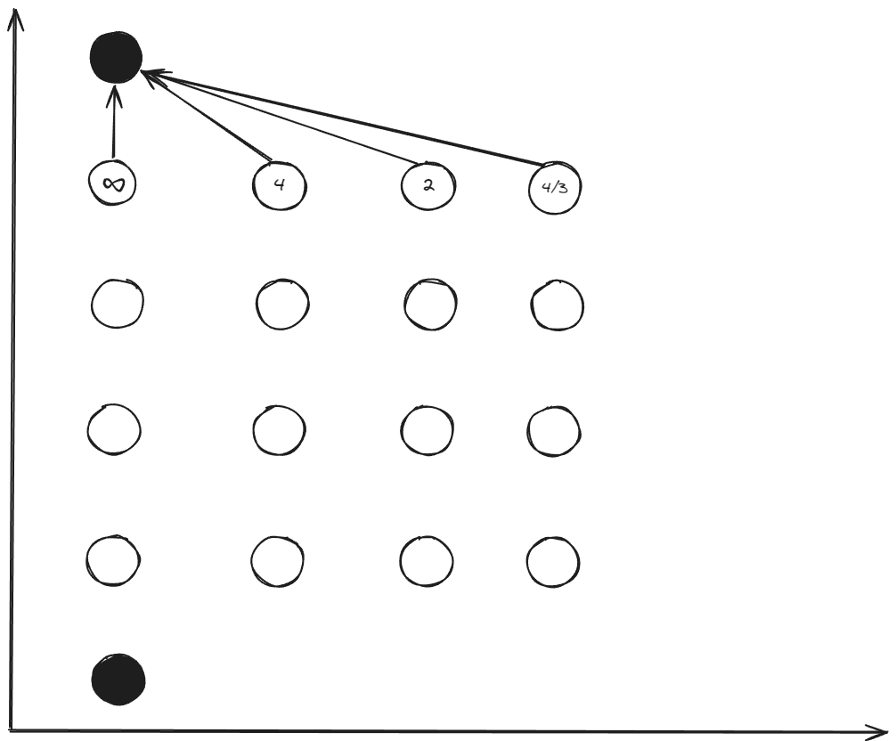
Step 2: Backward Recursion ($k = 5 \to 6$)

Starting from the final stage:

$$k = 6: x_{[6]} = [10 \; 0]^T$$ $$k = 5: x_{[5_i]} = [8 \; v_i]^T, \quad i = 1,2,3,4$$

Calculate transitions:

For $x_{[5_1]} = [8 \; 0]^T \to x_{[6]} = [10 \; 0]^T$:

$$\Delta t_{[5_1 \to 6]} = \frac{4}{0+0} = \infty$$

For $x_{[5_2]} = [8 \; 1]^T \to x_{[6]} = [10 \; 0]^T$:

$$\Delta t_{[5_2 \to 6]} = \frac{4}{1+0} = 4$$ $$u_{[5_2 \to 6]} = \frac{0-1}{4} = -\frac{1}{4}$$

For $x_{[5_3]} = [8 \; 2]^T \to x_{[6]} = [10 \; 0]^T$:

$$\Delta t_{[5_3 \to 6]} = \frac{4}{2+0} = 2$$ $$u_{[{5_3}{\to}{6}]} = \frac{0-4}{4} = -1$$

For $x_{[5_4]} = [8 \; 3]^T \to x_{[6]} = [10 \; 0]^T$:

$$\Delta t_{[5_4 \to 6]} = \frac{4}{3+0} = \frac{4}{3}$$ $$u_{[5_4 \to 6]} = \frac{0-9}{4} = -\frac{9}{4}$$

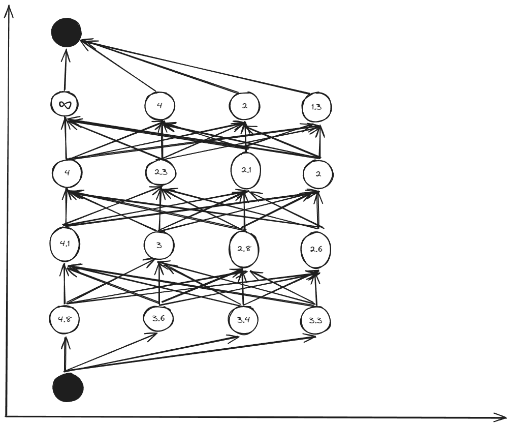
Cost-to-go values:

$$J_{[5_1 \to 6]}^* = \infty, \quad J_{[5_2 \to 6]}^* = 4, \quad J_{[5_3 \to 6]}^* = 2, \quad J_{[5_4 \to 6]}^* = \frac{4}{3}$$

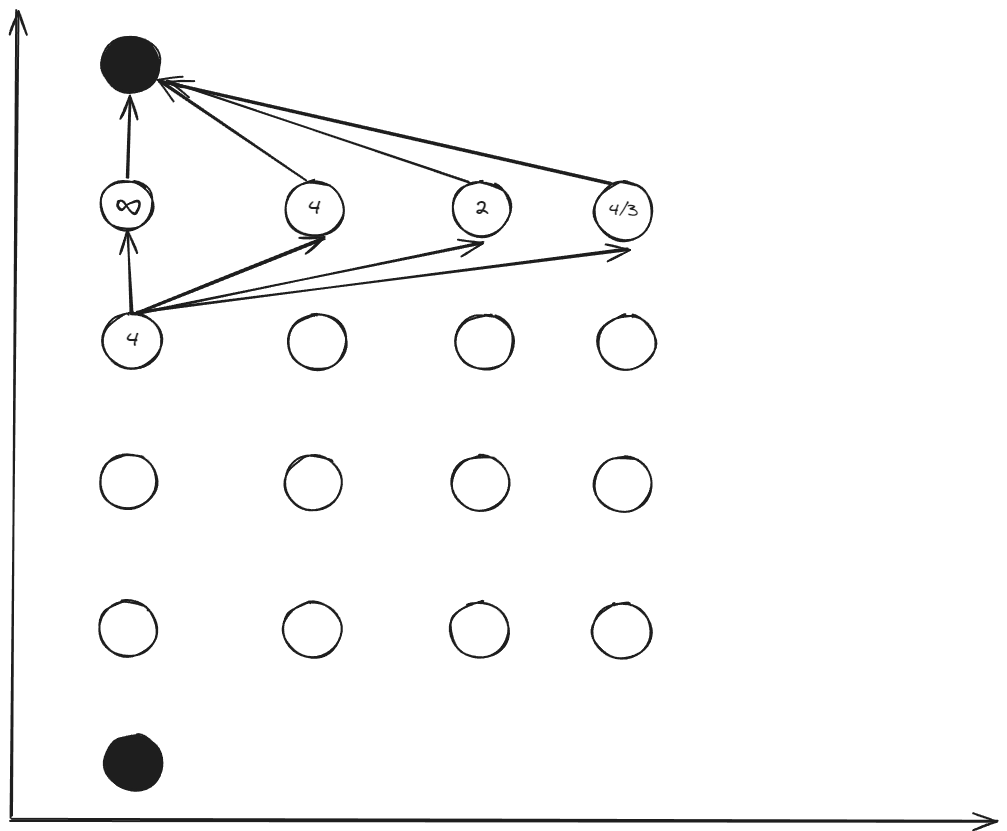
Step 3: Continue Backward ($k = 4 \to 5$)

For each node at stage 4, evaluate all possible transitions to stage 5.

Example for $x_{[4_1]} = [6 \; 0]^T$:

Evaluate transitions to all stage 5 nodes:

• $4_1 \to 5_1$: $\Delta t = \infty$ (infeasible)
• $4_1 \to 5_2$: $\Delta t = 4$, $u = \frac{1}{4}$
• $4_1 \to 5_3$: $\Delta t = 2$, $u = 1$
• $4_1 \to 5_4$: $\Delta t = \frac{4}{3}$, $u = \frac{9}{4}$ (violates constraint)

Optimal choice: $4_1 \to 5_3$ with total cost:

$$J_{[4_1]}^* = \Delta t_{[4_1 \to 5_3]} + J_{[5_3]}^* = 2 + 2 = 4$$

Step 4: Complete Backward Calculation

Continue this process for all stages until reaching the initial state.

Final cost-to-go table:

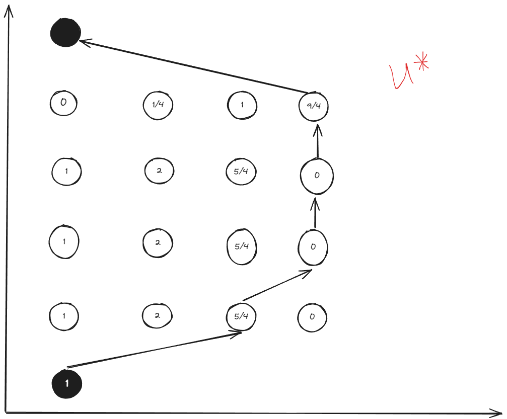
Optimal control policy table:

Key Advantages of Dynamic Programming

1. Computational Efficiency

• Brute force: $O(n^{N-1})$ exponential complexity
• Dynamic programming: $O(N \cdot n^2)$ polynomial complexity

2. Optimal Substructure

At each stage $k$, we compute all possible actions for each node but retain only the optimal result. This satisfies the Bellman principle: whatever happened before, the optimal path from the current node to the end has been determined.

3. Offline Computation

The entire control policy can be computed offline and stored in lookup tables for real-time implementation.

MATLAB Implementation

clear; close all;
set(0,'DefaultAxesFontName','Times New Roman')
set(0,'DefaultAxesFontSize',22)

% Problem parameters
h_init = 0; v_init = 0;
h_final = 10; v_final = 0;
h_min = 0; h_max = 10; N_h = 5;
v_min = 0; v_max = 3; N_v = 3;
u_min = -3; u_max = 2;

% Create state arrays
Hd = h_min:(h_max-h_min)/N_h:h_max;
Vd = v_min:(v_max-v_min)/N_v:v_max;

% Initialize cost-to-go and input matrices
J_costtogo = zeros(N_h+1, N_v+1);
Input_acc = zeros(N_h+1, N_v+1);

% Backward dynamic programming
for k = 2:N_h
    if k == 2
        % Final stage: transition to target
        v_avg = 0.5*(v_final + Vd);
        T_delta = (h_max-h_min)./(N_h * v_avg);
        acc = (0 - Vd)./T_delta;
    else
        % Intermediate stages
        [Vd_x, Vd_y] = meshgrid(Vd, Vd);
        v_avg = 0.5*(Vd_x + Vd_y);
        T_delta = (h_max-h_min)./(N_h * v_avg);
        acc = (Vd_y - Vd_x)./T_delta;
    end
    
    % Apply constraints
    J_temp = T_delta;
    [acc_x, acc_y] = find(acc < u_min | acc > u_max);
    J_temp(sub2ind(size(acc), acc_x, acc_y)) = inf;
    
    if k > 2
        J_temp = J_temp + meshgrid(J_costtogo(k-1,:))';
        [J_costtogo(k,:), l] = min(J_temp);
        Input_acc(k,:) = acc(sub2ind(size(J_temp), l, 1:length(l)));
    else
        J_costtogo(k,:) = J_temp;
        Input_acc(k,:) = acc;
    end
end

% Forward simulation using optimal policy
h_plot = zeros(N_h+1,1); v_plot = zeros(N_h+1,1); acc_plot = zeros(N_h,1);
h_plot(1) = h_init; v_plot(1) = v_init;

for k = 1:N_h
    [~, h_idx] = min(abs(h_plot(k) - Hd));
    [~, v_idx] = min(abs(v_plot(k) - Vd));
    acc_plot(k) = Input_acc(N_h+2-h_idx, v_idx);
    v_plot(k+1) = sqrt(2*(h_max-h_min)/N_h*acc_plot(k) + v_plot(k)^2);
    h_plot(k+1) = h_plot(k) + (h_max-h_min)/N_h;
end

% Plot results
figure;
plot(v_plot, h_plot, '--^', 'LineWidth', 2, 'MarkerSize', 8);
grid on; xlabel('Velocity (m/s)'); ylabel('Height (m)');
title('Optimal Trajectory');

Simulation Results

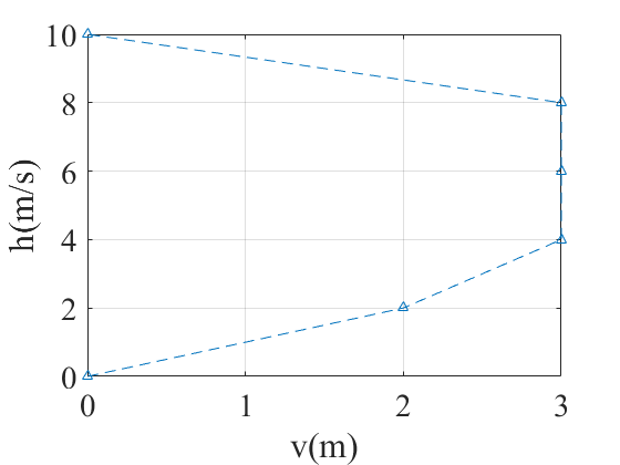
The optimal trajectory shows the drone accelerating initially to gain speed, then decelerating to reach zero velocity at the target height, all while respecting the input and state constraints.

Advantages and Limitations

Advantages

1. Guaranteed optimality for the discretized problem
2. Polynomial complexity vs. exponential brute force
3. Offline computation enables real-time implementation
4. Handles constraints naturally
5. Provides complete policy for all states

Limitations

1. Curse of dimensionality: Exponential growth with state dimension
2. Discretization errors: Approximate solution for continuous problems
3. Memory requirements: Must store value function/policy
4. Fixed grid: May miss optimal continuous solutions

Extensions and Applications

1. Stochastic Dynamic Programming

Handle uncertain dynamics and disturbances by considering expected costs.

2. Approximate Dynamic Programming

Use function approximation to handle high-dimensional problems.

3. Real-time Applications

• Model Predictive Control: Apply DP in receding horizon
• Reinforcement Learning: Learn value functions through experience
• Game Theory: Multi-agent optimal control

References

1. Optimal Control by DR_CAN
2. Wang, T. (2023). 控制之美 (卷2). Tsinghua University Press.
3. Rakovic, S. V., & Levine, W. S. (2018). Handbook of Model Predictive Control.
4. Bellman, R. (1957). Dynamic Programming. Princeton University Press.
5. Bertsekas, D. P. (2017). Dynamic Programming and Optimal Control (4th ed.). Athena Scientific.