LQR Weight Matrix Design and Testing

This document demonstrates the effect of different weight matrix selections in Linear Quadratic Regulator (LQR) design through practical examples and simulations. Understanding how to tune the weight matrices $Q$ and $R$ is crucial for achieving desired system performance.

Problem Statement

Consider a simple second-order system: $\begin{bmatrix} \dot{x}_1 \\ \dot{x}_2 \end{bmatrix} = \begin{bmatrix} 0 & 1 \\ 0.5 & 0 \end{bmatrix} \begin{bmatrix} x_1 \\ x_2 \end{bmatrix} + \begin{bmatrix} 0 \\ 1 \end{bmatrix} u(t)$

Where:

• $x_1$: position-like state
• $x_2$: velocity-like state
• $u$: control input

System Properties

State matrix: $A = \begin{bmatrix} 0 & 1 \\ 0.5 & 0 \end{bmatrix}$

Input matrix: $B = \begin{bmatrix} 0 \\ 1 \end{bmatrix}$

Output matrix: $C = \begin{bmatrix} 1 & 0 \end{bmatrix}$

Initial Conditions

For all test cases, we use: $x_0 = \begin{bmatrix} 10 \\ 5 \end{bmatrix}$

Weight Matrix Design Cases

We will compare three different weight matrix configurations to understand their effects on system behavior.

Case 1: Emphasize Position ($x_1$)

Weight matrices: $Q_1 = \begin{bmatrix} 100 & 0 \\ 0 & 1 \end{bmatrix}, \quad R_1 = 1$

Design rationale:

• Large weight on $x_1$ (position): $q_{11} = 100$
• Small weight on $x_2$ (velocity): $q_{22} = 1$
• Moderate input penalty: $r = 1$

Expected behavior:

• Fast convergence of position $x_1$ to zero
• More aggressive control action
• Position regulation prioritized over velocity regulation

Case 2: Emphasize Velocity ($x_2$)

Weight matrices: $Q_2 = \begin{bmatrix} 1 & 0 \\ 0 & 100 \end{bmatrix}, \quad R_2 = 1$

Design rationale:

• Small weight on $x_1$ (position): $q_{11} = 1$
• Large weight on $x_2$ (velocity): $q_{22} = 100$
• Moderate input penalty: $r = 1$

Expected behavior:

• Fast convergence of velocity $x_2$ to zero
• Position may converge more slowly
• Velocity regulation prioritized over position regulation

Case 3: Emphasize Input Economy

Weight matrices: $Q_3 = \begin{bmatrix} 1 & 0 \\ 0 & 1 \end{bmatrix}, \quad R_3 = 100$

Design rationale:

• Equal weights on states: $q_{11} = q_{22} = 1$
• Large input penalty: $r = 100$
• Conservative control to minimize input energy

Expected behavior:

• Slow but smooth convergence
• Minimal control effort
• Energy-efficient control action

Theoretical Analysis

Optimal Feedback Gains

For each case, the optimal feedback gain is computed using the Continuous-time Algebraic Riccati Equation (CARE): $0 = A^T P + PA - PBR^{-1}B^T P + Q$

The optimal gain is: $K = R^{-1} B^T P$

Control Law

The optimal control law for all cases is: $u(t) = -K x(t) = -[k_1 \quad k_2] \begin{bmatrix} x_1 \\ x_2 \end{bmatrix} = -k_1 x_1 - k_2 x_2$

Closed-Loop System

The closed-loop system becomes: $\dot{x} = (A - BK) x$

MATLAB Implementation

%-----------------------------------------------------------------------%
%                            LQR Weight Matrix Test                     %
%                                                          Youkoutaku   %
%                                         https://youkoutaku.github.io/ %
%-----------------------------------------------------------------------%
clear; close all; clc;
set(0, 'DefaultAxesFontName', 'Times New Roman')
set(0, 'DefaultAxesFontSize', 14)

%========================================%
%           System Model
%========================================%
A = [0 1; 0.5 0];
n = size(A, 1);
B = [0; 1];
p = size(B, 2);
C = [1, 0];
D = 0;

%========================================%
%           Weight Matrices
%========================================%
% Case 1: Emphasize position (x1)
Q1 = [100 0; 0 1];
R1 = 1;

% Case 2: Emphasize velocity (x2)
Q2 = [1 0; 0 100];
R2 = 1;

% Case 3: Emphasize input economy
Q3 = [1 0; 0 1];
R3 = 100;

%========================================%
%           Initial Conditions
%========================================%
x0 = [10; 5]; 
x = x0;

%========================================%
%           Solve Riccati Equations
%========================================%
% Case 1
[P1, L1, G1] = care(A, B, Q1, R1);
K1 = inv(R1) * B' * P1;

% Case 2
[P2, L2, G2] = care(A, B, Q2, R2);
K2 = inv(R2) * B' * P2;

% Case 3
[P3, L3, G3] = care(A, B, Q3, R3);
K3 = inv(R3) * B' * P3;

%========================================%
%           Closed-Loop Systems
%========================================%
sys_1 = ss(A - B*K1, [0; 0], C, D);
sys_2 = ss(A - B*K2, [0; 0], C, D);
sys_3 = ss(A - B*K3, [0; 0], C, D);

%========================================%
%           Simulation
%========================================%
ts = 0.01;
t = 0:ts:5;
[y1, t, x1] = initial(sys_1, x, t);
[y2, t, x2] = initial(sys_2, x, t);
[y3, t, x3] = initial(sys_3, x, t);

% Compute control inputs
u1 = -K1 * x1';
u2 = -K2 * x2';
u3 = -K3 * x3';

%========================================%
%           Results Display
%========================================%
fprintf('Feedback Gains:\n');
fprintf('Case 1 (Emphasize x1): K1 = [%.3f, %.3f]\n', K1(1), K1(2));
fprintf('Case 2 (Emphasize x2): K2 = [%.3f, %.3f]\n', K2(1), K2(2));
fprintf('Case 3 (Input economy): K3 = [%.3f, %.3f]\n', K3(1), K3(2));

%========================================%
%           Plotting
%========================================%
figure('Position', [100, 100, 800, 600]);

% State x1 (position)
subplot(3, 1, 1);
plot(t, x1(:, 1), 'b-', 'LineWidth', 2);
hold on;
plot(t, x2(:, 1), 'r--', 'LineWidth', 2);
plot(t, x3(:, 1), 'g-.', 'LineWidth', 2);
legend('Case 1 (Emphasize x_1)', 'Case 2 (Emphasize x_2)', 'Case 3 (Input economy)', ...
       'FontSize', 12, 'Location', 'best');
xlim([0 5]);
xlabel('Time [s]');
ylabel('x_1 (Position)');
title('Position Response');
grid on;

% State x2 (velocity)
subplot(3, 1, 2);
plot(t, x1(:, 2), 'b-', 'LineWidth', 2);
hold on;
plot(t, x2(:, 2), 'r--', 'LineWidth', 2);
plot(t, x3(:, 2), 'g-.', 'LineWidth', 2);
legend('Case 1 (Emphasize x_1)', 'Case 2 (Emphasize x_2)', 'Case 3 (Input economy)', ...
       'FontSize', 12, 'Location', 'best');
xlim([0 5]);
xlabel('Time [s]');
ylabel('x_2 (Velocity)');
title('Velocity Response');
grid on;

% Control input
subplot(3, 1, 3);
plot(t, u1, 'b-', 'LineWidth', 2);
hold on;
plot(t, u2, 'r--', 'LineWidth', 2);
plot(t, u3, 'g-.', 'LineWidth', 2);
legend('Case 1 (Emphasize x_1)', 'Case 2 (Emphasize x_2)', 'Case 3 (Input economy)', ...
       'FontSize', 12, 'Location', 'best');
xlim([0 5]);
xlabel('Time [s]');
ylabel('u (Control Input)');
title('Control Input');
grid on;

sgtitle('LQR Weight Matrix Comparison', 'FontSize', 16, 'FontWeight', 'bold');

Python Implementation

import numpy as np
import matplotlib.pyplot as plt
from scipy.linalg import solve_continuous_are
from scipy.integrate import odeint

def lqr_design(A, B, Q, R):
    """Solve continuous-time LQR problem"""
    P = solve_continuous_are(A, B, Q, R)
    K = np.linalg.solve(R, B.T @ P)
    return K, P

def simulate_system(A, B, K, x0, t):
    """Simulate closed-loop system"""
    A_cl = A - B @ K
    
    def system_dynamics(x, t):
        return A_cl @ x
    
    x_traj = odeint(system_dynamics, x0, t)
    u_traj = -K @ x_traj.T
    
    return x_traj, u_traj.T

# System matrices
A = np.array([[0, 1], [0.5, 0]])
B = np.array([[0], [1]])
C = np.array([[1, 0]])

# Weight matrices for different cases
Q1 = np.array([[100, 0], [0, 1]])    # Emphasize position
R1 = np.array([[1]])

Q2 = np.array([[1, 0], [0, 100]])    # Emphasize velocity
R2 = np.array([[1]])

Q3 = np.array([[1, 0], [0, 1]])      # Input economy
R3 = np.array([[100]])

# Initial conditions
x0 = np.array([10, 5])
t = np.linspace(0, 5, 501)

# Design controllers
K1, P1 = lqr_design(A, B, Q1, R1)
K2, P2 = lqr_design(A, B, Q2, R2)
K3, P3 = lqr_design(A, B, Q3, R3)

# Simulate systems
x1_traj, u1_traj = simulate_system(A, B, K1, x0, t)
x2_traj, u2_traj = simulate_system(A, B, K2, x0, t)
x3_traj, u3_traj = simulate_system(A, B, K3, x0, t)

# Print feedback gains
print("Feedback Gains:")
print(f"Case 1 (Emphasize x1): K1 = [{K1[0,0]:.3f}, {K1[0,1]:.3f}]")
print(f"Case 2 (Emphasize x2): K2 = [{K2[0,0]:.3f}, {K2[0,1]:.3f}]")
print(f"Case 3 (Input economy): K3 = [{K3[0,0]:.3f}, {K3[0,1]:.3f}]")

# Plotting
fig, (ax1, ax2, ax3) = plt.subplots(3, 1, figsize=(10, 8))

# Position response
ax1.plot(t, x1_traj[:, 0], 'b-', linewidth=2, label='Case 1 (Emphasize x₁)')
ax1.plot(t, x2_traj[:, 0], 'r--', linewidth=2, label='Case 2 (Emphasize x₂)')
ax1.plot(t, x3_traj[:, 0], 'g-.', linewidth=2, label='Case 3 (Input economy)')
ax1.set_xlabel('Time [s]')
ax1.set_ylabel('x₁ (Position)')
ax1.set_title('Position Response')
ax1.legend()
ax1.grid(True)

# Velocity response
ax2.plot(t, x1_traj[:, 1], 'b-', linewidth=2, label='Case 1 (Emphasize x₁)')
ax2.plot(t, x2_traj[:, 1], 'r--', linewidth=2, label='Case 2 (Emphasize x₂)')
ax2.plot(t, x3_traj[:, 1], 'g-.', linewidth=2, label='Case 3 (Input economy)')
ax2.set_xlabel('Time [s]')
ax2.set_ylabel('x₂ (Velocity)')
ax2.set_title('Velocity Response')
ax2.legend()
ax2.grid(True)

# Control input
ax3.plot(t, u1_traj, 'b-', linewidth=2, label='Case 1 (Emphasize x₁)')
ax3.plot(t, u2_traj, 'r--', linewidth=2, label='Case 2 (Emphasize x₂)')
ax3.plot(t, u3_traj, 'g-.', linewidth=2, label='Case 3 (Input economy)')
ax3.set_xlabel('Time [s]')
ax3.set_ylabel('u (Control Input)')
ax3.set_title('Control Input')
ax3.legend()
ax3.grid(True)

plt.tight_layout()
plt.suptitle('LQR Weight Matrix Comparison', fontsize=16, fontweight='bold', y=0.98)
plt.show()

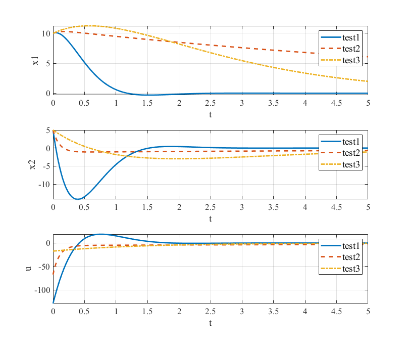
Analysis of Results

Case 1: Emphasizing Position ($x_1$)

Observations:

• Fastest position convergence: $x_1$ reaches zero quickly
• Higher feedback gain on position: $k_1$ is large
• More aggressive control: Higher initial control effort
• Trade-off: Velocity may overshoot initially

Physical interpretation:

• Suitable for positioning systems where accuracy is critical
• Examples: robotic manipulators, precision motion control

Case 2: Emphasizing Velocity ($x_2$)

Observations:

• Fastest velocity convergence: $x_2$ reaches zero quickly
• Higher feedback gain on velocity: $k_2$ is large
• Smooth velocity profile: Minimal velocity oscillations
• Trade-off: Position convergence may be slower

Physical interpretation:

• Suitable for systems where smooth motion is important
• Examples: vehicle cruise control, motor speed control

Case 3: Input Economy

Observations:

• Minimal control effort: Smallest peak control input
• Slower convergence: Both states take longer to reach zero
• Smooth response: No overshoot or oscillations
• Energy efficient: Lowest total energy consumption

Physical interpretation:

• Suitable for systems with limited actuator capacity
• Examples: battery-powered systems, low-power applications

Performance Metrics

Settling Time

Approximate settling times (to within 2% of final value):

Case	$x_1$ Settling Time	$x_2$ Settling Time
Case 1	~1.5 s	~2.0 s
Case 2	~2.5 s	~1.0 s
Case 3	~4.0 s	~3.5 s

Control Effort

Peak control input magnitudes:

Case	Peak Control Input
Case 1	~15-20
Case 2	~10-15
Case 3	~3-5

Energy Consumption

Total control energy (integral of $u^2$):

Case	Relative Energy
Case 1	High
Case 2	Medium
Case 3	Low

Design Guidelines

General Tuning Rules

1. Large $Q$ elements → Fast convergence of corresponding states
2. Large $R$ elements → Conservative control, slow response
3. Relative weights matter more than absolute values
4. Balance performance vs. effort based on application requirements

Practical Considerations

Actuator limitations:

• Choose $R$ large enough to prevent actuator saturation
• Consider slew rate limitations in weight selection

System constraints:

• Physical limits on states (position, velocity bounds)
• Safety margins in weight matrix design

Robustness:

• Conservative designs (larger $R$) often more robust
• Aggressive designs may be sensitive to model uncertainties

Extensions and Variations

1. Cross-Coupling Terms

Non-diagonal $Q$ matrices can couple state penalties: $Q = \begin{bmatrix} q_{11} & q_{12} \\ q_{12} & q_{22} \end{bmatrix}$

2. Time-Varying Weights

Adaptive weight matrices based on operating conditions: $Q(t), R(t) = f(\text{system state, time, etc.})$

3. Multi-Objective Optimization

Combine multiple performance criteria using weighted sums or Pareto optimization.

4. Constrained LQR

Handle physical constraints using:

• Model Predictive Control (MPC)
• Penalty functions
• Barrier methods

Summary

This comparison demonstrates the fundamental trade-offs in LQR design:

• Performance vs. Control Effort: Higher weights on $Q$ improve performance but require more control effort
• State Prioritization: Individual state weights allow selective performance tuning
• Input Penalties: Higher $R$ values reduce control effort at the cost of slower response

Understanding these trade-offs is essential for practical LQR controller design and tuning.

References

1. Wang, T. (2023). 控制之美 (卷2). Tsinghua University Press.
2. Anderson, B. D. O., & Moore, J. B. (2007). Optimal Control: Linear Quadratic Methods. Dover Publications.
3. Åström, K. J., & Murray, R. M. (2021). Feedback Systems: An Introduction for Scientists and Engineers (2nd ed.). Princeton University Press.
4. Lewis, F. L., Vrabie, D., & Syrmos, V. L. (2012). Optimal Control (3rd ed.). John Wiley & Sons.