Titanic - Machine Learning from Disaster

Problem and Background

Titanic - Machine Learning from Disaster

Problem: Create a machine learning model to predict which passengers survived the Titanic disaster.

Background: According to the Kaggle competition "Titanic - Machine Learning from Disaster" description: "On April 15, 1912, during her maiden voyage, the widely considered 'unsinkable' RMS Titanic sank after colliding with an iceberg. Unfortunately, there weren't enough lifeboats for everyone onboard, resulting in the death of 1502 out of 2224 passengers and crew."

While there was an element of luck involved, certain groups of people were more likely to survive than others, such as women, children, and the upper-class.

Machine Learning Final Report Name: YANG GUANGZE Student ID: 20T1126N

More about machine learning | Github

Analysis Overview

# Import libraries
import numpy as np 
import pandas as pd 
import matplotlib.pyplot as plt 
import seaborn as sns 
%matplotlib inline

# Suppress warnings
import warnings
warnings.filterwarnings("ignore")

# Set Jupyter Notebook display options
pd.set_option("display.max_columns", 100) 
pd.set_option("display.max_rows", 100)

# Load data
train_df = pd.read_csv("./train.csv") 
test_df = pd.read_csv("./test.csv") 
train_df.head(10) # Display first 10 rows

PassengerId	Survived	Pclass	Name	Sex	Age	SibSp	Parch	Ticket	Fare	Cabin	Embarked
PassengerId	Survived	Pclass	Name	Sex	Age	SibSp	Parch	Ticket	Fare	Cabin	Embarked
-------------	----------	--------	------	-----	-----	-------	-------	--------	------	-------	----------
0	1	0	3	Braund, Mr. Owen Harris	male	22.0	1	0	A/5 21171	7.2500	NaN
1	2	1	1	Cumings, Mrs. John Bradley (Florence Briggs Th...)	female	38.0	1	0	PC 17599	71.2833	C85
2	3	1	3	Heikkinen, Miss. Laina	female	26.0	0	0	STON/O2. 3101282	7.9250	NaN
3	4	1	1	Futrelle, Mrs. Jacques Heath (Lily May Peel)	female	35.0	1	0	113803	53.1000	C123
4	5	0	3	Allen, Mr. William Henry	male	35.0	0	0	373450	8.0500	NaN
5	6	0	3	Moran, Mr. James	male	NaN	0	0	330877	8.4583	NaN
6	7	0	1	McCarthy, Mr. Timothy J	male	54.0	0	0	17463	51.8625	E46
7	8	0	3	Palsson, Master. Gosta Leonard	male	2.0	3	1	349909	21.0750	NaN
8	9	1	3	Johnson, Mrs. Oscar W (Elisabeth Vilhelmina Berg)	female	27.0	0	2	347742	11.1333	NaN
9	10	1	2	Nasser, Mrs. Nicholas (Adele Achem)	female	14.0	1	0	237736	30.0708	NaN

# Check data size
print(train_df.shape) 
print(test_df.shape)

(891, 12) (418, 11)

Analysis Description

The data contains one target variable Survived and explanatory variables: PassengerId, Pclass, Name, Sex, Age, SibSp, Parch, Ticket, Fare, Cabin, and Embarked.

In English terms, these represent: passenger ID, passenger class, passenger name, gender, age, number of siblings/spouses aboard, number of parents/children aboard, ticket number, fare, cabin number, and port of embarkation.

This analysis focuses on using these explanatory variables to predict the target variable Survived through machine learning classification.

The dataset consists of 891 training samples and 418 test samples.

The analysis covers:

1. Understanding the training data
2. Feature engineering
3. Machine learning
4. Final Kaggle results

1. Understanding the Training Data

1.1 Data Verification

Examining data types and missing values to identify features that require preprocessing.

train_df.dtypes # Display data types
train_df.info() # Display data details

<class 'pandas.core.frame.DataFrame'> RangeIndex: 891 entries, 0 to 890 Data columns (total 12 columns):

Column Non-Null Count Dtype

---

0 PassengerId 891 non-null int64
1 Survived 891 non-null int64
2 Pclass 891 non-null int64
3 Name 891 non-null object 4 Sex 891 non-null object 5 Age 714 non-null float64 6 SibSp 891 non-null int64
7 Parch 891 non-null int64
8 Ticket 891 non-null object 9 Fare 891 non-null float64 10 Cabin 204 non-null object 11 Embarked 889 non-null object dtypes: float64(2), int64(5), object(5) memory usage: 83.7+ KB

test_df.dtypes # Display data types
test_df.info() # Display data details

<class 'pandas.core.frame.DataFrame'> RangeIndex: 418 entries, 0 to 417 Data columns (total 11 columns):

Column Non-Null Count Dtype

---

0 PassengerId 418 non-null int64
1 Pclass 418 non-null int64
2 Name 418 non-null object 3 Sex 418 non-null object 4 Age 332 non-null float64 5 SibSp 418 non-null int64
6 Parch 418 non-null int64
7 Ticket 418 non-null object 8 Fare 417 non-null float64 9 Cabin 91 non-null object 10 Embarked 418 non-null object dtypes: float64(2), int64(4), object(5) memory usage: 36.0+ KB

Key findings:

1. Data types: Name, Sex, Ticket, Cabin, Embarked are object types requiring feature engineering (dummy variable conversion).

2. Missing data: Age and Fare have missing values requiring imputation.

3. Cabin feature: Has significant missing data, so it's better not to treat it as an important feature.

1.2 Data Distribution and Target Variable Relationships

Analyzing variable distributions to understand each feature's relationship with survival.

1.2.1 Target Variable Survived

# Survival rate in training data (1: survived, 0: died)
train_df["Survived"].mean()

0.3838383838383838

The survival rate in the training data is approximately 38%.

1.2.2 Feature Pclass

Passenger class is expected to significantly impact survival due to socioeconomic status differences.

# Element frequency
train_df["Pclass"].value_counts()

3 491 1 216 2 184 Name: Pclass, dtype: int64

# Survival count by Pclass
import seaborn as sns 
sns.countplot(data=train_df, x="Pclass", hue="Survived");

# Survival rate by Pclass
train_df["Survived"].groupby(train_df["Pclass"]).mean()

Pclass 1 0.629630 2 0.472826 3 0.242363 Name: Survived, dtype: float64

Result: Survival rates vary significantly by passenger class. Higher class passengers (1>2>3) have much better survival rates. Pclass is a very important variable.

1.2.3 Feature Sex

Gender is expected to significantly impact survival due to the "ladies first" cultural norm.

# Survival count by Sex (1: survived, 0: died)
sns.countplot(data=train_df, x="Sex", hue="Survived");

# Element frequency
train_df["Sex"].value_counts()

male 577 female 314 Name: Sex, dtype: int64

# Survival rate by Sex
train_df["Survived"].groupby(train_df["Sex"]).mean()

Sex female 0.742038 male 0.188908 Name: Survived, dtype: float64

Result: As expected, females have much higher survival rates than males.

# Sex distribution by Pclass
sns.countplot(data=train_df, x="Sex", hue="Pclass");

This chart shows that even though males are more concentrated in lower classes, females still have higher survival rates, confirming a direct gender effect (female > male), potentially more influential than class.

1.2.4 Feature Age

Age is expected to significantly impact survival due to the "children first" principle.

# Extract Age data
Age0 = train_df[train_df["Survived"]==0]["Age"] 
Age1 = train_df[train_df["Survived"]==1]["Age"]

# Histogram
plt.hist([Age0, Age1], bins=8, label=["0: Death", "1: Survive"]) 
plt.legend() 
plt.xlabel("Age");

Result: As expected, younger passengers have higher survival rates.

# Age and Sex relationship
Age2 = train_df[train_df["Sex"]=="male"]["Age"] 
Age3 = train_df[train_df["Sex"]=="female"]["Age"]

# Histogram
plt.hist([Age2, Age3], bins=8, label=["male", "female"]) 
plt.legend() 
plt.xlabel("Age");

# Age and Pclass relationship
Age4 = train_df[train_df["Pclass"]==1]["Age"] 
Age5 = train_df[train_df["Pclass"]==2]["Age"]
Age6 = train_df[train_df["Pclass"]==3]["Age"]

# Histogram
plt.hist([Age4, Age5, Age6], bins=8, label=["Pclass:1", "Pclass:2","Pclass:3"]) 
plt.legend() 
plt.xlabel("Age");

Since there's no significant age bias across classes and genders, the higher survival rate of younger passengers is considered a direct age effect.

1.2.5 Features SibSp and Parch

The number of siblings, spouses, parents, and children aboard is expected to have minimal impact on survival rates.

# Survival rate by SibSp
train_df["Survived"].groupby(train_df["SibSp"]).mean()

SibSp 0 0.345395 1 0.535885 2 0.464286 3 0.250000 4 0.166667 5 0.000000 8 0.000000 Name: Survived, dtype: float64

# Element frequency
train_df["SibSp"].value_counts()

0 608 1 209 2 28 4 18 3 16 8 7 5 5 Name: SibSp, dtype: int64

# SibSp histogram
SibSp0 = train_df[train_df["Survived"]==0]["SibSp"] 
SibSp1 = train_df[train_df["Survived"]==1]["SibSp"]
plt.hist([SibSp0, SibSp1], bins=8, label=["0: Death", "1: Survive"]) 
plt.legend() 
plt.xlabel("SibSp");

# Survival rate by Parch
train_df["Survived"].groupby(train_df["Parch"]).mean()

Parch 0 0.343658 1 0.550847 2 0.500000 3 0.600000 4 0.000000 5 0.200000 6 0.000000 Name: Parch, dtype: float64

# Element frequency
train_df["Parch"].value_counts()

0 678 1 118 2 80 5 5 3 5 4 4 6 1 Name: Parch, dtype: int64

# Parch histogram
Parch0 = train_df[train_df["Survived"]==0]["Parch"] 
Parch1 = train_df[train_df["Survived"]==1]["SibSp"]
plt.hist([Parch0, Parch1], bins=6, label=["0: Death", "1: Survive"]) 
plt.legend() 
plt.xlabel("Parch");

Result: Due to frequency distribution, passengers with more family members are fewer, making the data less reliable. The relationship between family size and survival rate is not linear. However, having family aboard appears to affect survival rates.

For features SibSp and Parch, creating a new feature "Family" to indicate family presence could improve model accuracy.

1.2.6 Feature Fare

Fare is expected to slightly impact survival rates as it also represents social class.

# Fare histogram
Fare0 = train_df[train_df["Survived"]==0]["Fare"] 
Fare1 = train_df[train_df["Survived"]==1]["Fare"]
plt.hist([Fare0, Fare1], bins=8, label=["0: Death", "1: Survive"]) 
plt.legend() 
plt.xlabel("Fare");

Result: As expected, passengers with higher fares have better survival chances.

# Fare and Pclass relationship
Fare2 = train_df[train_df["Pclass"]==1]["Fare"] 
Fare3 = train_df[train_df["Pclass"]==2]["Fare"]
Fare4 = train_df[train_df["Pclass"]==3]["Fare"]
plt.hist([Fare2, Fare3, Fare4], bins=8, label=["Pclass:1", "Pclass:2","Pclass:3"]) 
plt.legend() 
plt.xlabel("Fare");

Since fare shows clear bias by class, the fare effect is considered an indirect effect of class. To improve model accuracy, the Fare feature weight should be reduced.

1.2.7 Features Name, Ticket, Cabin, Embarked

Name, ticket number, cabin number, and embarkation port are expected to have minimal impact on survival rates due to their diverse string nature without clear patterns.

# Check Name data
train_df["Name"].head()

0 Braund, Mr. Owen Harris 1 Cumings, Mrs. John Bradley (Florence Briggs Th... 2 Heikkinen, Miss. Laina 3 Futrelle, Mrs. Jacques Heath (Lily May Peel) 4 Allen, Mr. William Henry Name: Name, dtype: object

# Name frequency
train_df["Name"].value_counts()

Braund, Mr. Owen Harris 1 Boulos, Mr. Hanna 1 Frolicher-Stehli, Mr. Maxmillian 1 Gilinski, Mr. Eliezer 1 Murdlin, Mr. Joseph 1 .. Kelly, Miss. Anna Katherine "Annie Kate" 1 McCoy, Mr. Bernard 1 Johnson, Mr. William Cahoone Jr 1 Keane, Miss. Nora A 1 Dooley, Mr. Patrick 1 Name: Name, Length: 891, dtype: int64

# Check Ticket data
train_df["Ticket"].head()

0 A/5 21171 1 PC 17599 2 STON/O2. 3101282 3 113803 4 373450 Name: Ticket, dtype: object

# Ticket frequency
train_df["Ticket"].value_counts()

347082 7 CA. 2343 7 1601 7 3101295 6 CA 2144 6 .. 9234 1 19988 1 2693 1 PC 17612 1 370376 1 Name: Ticket, Length: 681, dtype: int64

# Check Cabin data
train_df["Cabin"].head()

0 NaN 1 C85 2 NaN 3 C123 4 NaN Name: Cabin, dtype: object

# Cabin frequency
train_df["Cabin"].value_counts()

B96 B98 4 G6 4 C23 C25 C27 4 C22 C26 3 F33 3 .. E34 1 C7 1 C54 1 E36 1 C148 1 Name: Cabin, Length: 147, dtype: int64

# Survival rate by Embarked
train_df["Survived"].groupby(train_df["Embarked"]).mean()

Embarked C 0.553571 Q 0.389610 S 0.336957 Name: Embarked, dtype: float64

# Embarked frequency
train_df["Embarked"].value_counts()

S 644 C 168 Q 77 Name: Embarked, dtype: int64

# Embarked survival count
sns.countplot(data=train_df, x="Embarked", hue="Survived");

Result: Name, ticket number, and cabin number show expected patterns. However, embarkation port shows relationship with target variable.

Important features identified:

1. Pclass
2. Sex
3. Age
4. Embarked
5. Family (SibSp + Parch)

Excluding: PassengerId, Name, Ticket, Cabin

2. Feature Engineering

2.1 Combining Training and Test Data

# Fresh start
train_df = pd.read_csv("./train.csv") 
test_df = pd.read_csv("./test.csv")

# Remove unnecessary data
train_df = train_df.drop(['Name','Ticket', 'Cabin'], axis=1)
test_df = test_df.drop(['Name','Ticket', 'Cabin'], axis=1)

# Combine training and test data
all_df = pd.concat([train_df, test_df], sort=False) # No sorting

# Reset index numbers (train and test have duplicate indices)
all_df.reset_index(drop=True) # Remove old index

2.2 Categorical Variable Conversion

# Convert to dummy variables
all_df = pd.get_dummies(all_df, drop_first=True)

# Check missing values
all_df.isna().sum()

PassengerId 0 Survived 418 Pclass 0 Age 263 SibSp 0 Parch 0 Fare 1 Sex_male 0 Embarked_Q 0 Embarked_S 0 dtype: int64

2.3 Missing Value Imputation

# Fill missing values with mean
all_df["Age"] = all_df["Age"].fillna(all_df["Age"].mean()) 
all_df["Fare"] = all_df["Fare"].fillna(all_df["Fare"].mean())

2.4 Data Integration

# Create new Family variable
all_df["Family"] = np.where((all_df['SibSp'] == 0) & (all_df['Parch'] == 0), 0, 1)

# Verify new Family variable
all_df['Family']

0 1 1 1 2 0 3 1 4 0 .. 413 0 414 0 415 0 416 0 417 1 Name: Family, Length: 1309, dtype: int32

# Remove SibSp and Parch
all_df = all_df.drop(["SibSp", "Parch"], axis=1)

2.5 Data Separation

# Split back to train and test
train_df_2 = all_df[:len(train_df)] 
test_df_2 = all_df[len(train_df):]

# Separate features and target variable
train_X = train_df_2.drop(["Survived", "PassengerId"], axis=1) 
test_X = test_df_2.drop(["Survived", "PassengerId"], axis=1)
train_Y = train_df_2["Survived"]

train_X.shape, train_Y.shape, test_X.shape

((891, 7), (891,), (418, 7))

3. Machine Learning

The learning models include:

1. Decision Tree
2. Random Forest
3. Gradient Boosting
4. Ensemble Learning
5. Stacking

3.1 Decision Tree

# Decision Tree
from sklearn.tree import DecisionTreeClassifier 
from sklearn.model_selection import cross_val_score
MAX_DEPTH = 10
accuracy = np.zeros(MAX_DEPTH)

for depth in range(1, MAX_DEPTH+1):
    decision_tree = DecisionTreeClassifier(max_depth=depth)
    scores = cross_val_score(decision_tree, train_X, train_Y, cv=10)
    accuracy[depth-1] = np.mean(scores)
    
plt.plot(range(1, MAX_DEPTH+1), accuracy, '.-')

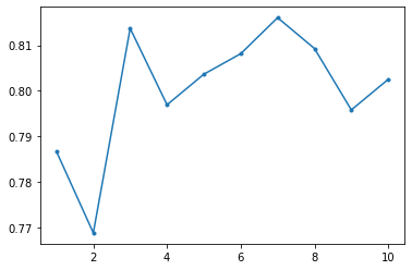
# Parameter optimization
decision_tree = DecisionTreeClassifier(max_depth=3)  # depth=3 to prevent overfitting
decision_tree.fit(train_X, train_Y)
Y_pred_dt = decision_tree.predict(test_X)

# Output prediction results
file = pd.read_csv("./gender_submission.csv") 
file["Survived"] = Y_pred_dt.astype(int)  # Convert to integer
file.to_csv("./submission_dt.csv", index=False)  # Don't overwrite index

3.2 Random Forest

# Random Forest
from sklearn.ensemble import RandomForestClassifier

X = train_X
Y = train_Y

MAX_DEPTH = 20
accuracy = np.zeros(MAX_DEPTH)

for depth in range(1, MAX_DEPTH+1):
    model_rf = RandomForestClassifier(n_estimators=500, max_depth=depth, random_state=1126)
    model_rf.fit(X, Y)
    model_rf.score(X, Y)
    scores = cross_val_score(model_rf, X, Y, cv=20)
    accuracy[depth-1] = np.mean(scores)
    
plt.plot(range(1, MAX_DEPTH+1), accuracy, '.-')

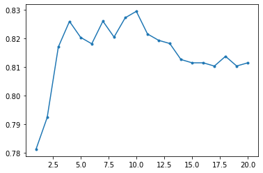
# Parameter optimization
model_rf = RandomForestClassifier(n_estimators=500, max_depth=4, random_state=1126)
model_rf.fit(train_X, train_Y)
Y_pred_rf = model_rf.predict(test_X)

file = pd.read_csv("./gender_submission.csv") 
file["Survived"] = Y_pred_rf.astype(int)
file.to_csv("./submission_rf.csv", index=False)

3.3 Gradient Boosting

from sklearn.ensemble import GradientBoostingClassifier

X = train_X
Y = train_Y

MAX_DEPTH = 10
accuracy = np.zeros(MAX_DEPTH)

for depth in range(1, MAX_DEPTH+1):
    model_gb = GradientBoostingClassifier(n_estimators=500, max_depth=depth, random_state=1234)
    scores = cross_val_score(model_gb, X, Y, cv=10)
    accuracy[depth-1] = np.mean(scores)
    
plt.plot(range(1, MAX_DEPTH+1), accuracy, '.-')

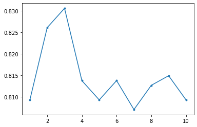
# Parameter optimization
model_gb = GradientBoostingClassifier(n_estimators=500, max_depth=3, random_state=1234)
model_gb.fit(train_X, train_Y)
Y_pred_gb = model_gb.predict(test_X)

file = pd.read_csv("./gender_submission.csv") 
file["Survived"] = Y_pred_gb.astype(int)
file.to_csv("./submission_gb.csv", index=False)

3.4 Ensemble Learning

model1 = RandomForestClassifier(n_estimators=500, random_state=1126, max_depth=4) 
model2 = RandomForestClassifier(n_estimators=500, random_state=9999, max_depth=4) 
model3 = GradientBoostingClassifier(n_estimators=500, random_state=1126, max_depth=3) 
model4 = GradientBoostingClassifier(n_estimators=500, random_state=9999, max_depth=3) 

# Training
model1.fit(train_X, train_Y) 
model2.fit(train_X, train_Y) 
model3.fit(train_X, train_Y) 
model4.fit(train_X, train_Y) 

# Testing
pred_test_Y1 = model1.predict(test_X) 
pred_test_Y2 = model2.predict(test_X) 
pred_test_Y3 = model3.predict(test_X) 
pred_test_Y4 = model4.predict(test_X) 

# Majority voting (average)
ensemble_Y = (pred_test_Y1 + pred_test_Y2 + pred_test_Y3 + pred_test_Y4) / 4

# Output prediction results
file = pd.read_csv("./gender_submission.csv") 
file["Survived"] = ensemble_Y.astype(int)
file.to_csv("./submission_ENS.csv", index=False)

3.5 Stacking

# Stacking
pred_train_Y1 = model1.predict(train_X)
pred_train_Y2 = model2.predict(train_X)
pred_train_Y3 = model3.predict(train_X)
pred_train_Y4 = model4.predict(train_X)
Ens_train_Y = np.array([pred_train_Y1, pred_train_Y2, pred_train_Y3, pred_train_Y4]).T

# Using SGD classifier instead of LinearClassifier (import issue)
# Stochastic Gradient Descent SGD
from sklearn.linear_model import SGDClassifier
model_boss = SGDClassifier()

X = Ens_train_Y
Y = train_Y

model_boss.fit(X, Y)

# Subordinate predictions
pred_test_Y1 = model1.predict(test_X)
pred_test_Y2 = model2.predict(test_X)
pred_test_Y3 = model3.predict(test_X)
pred_test_Y4 = model4.predict(test_X)
Ens_test_X = np.array([pred_test_Y1, pred_test_Y2, pred_test_Y3, pred_test_Y4]).T

# Boss prediction
pred_test_YBoss = model_boss.predict(Ens_test_X)

file = pd.read_csv("./gender_submission.csv") 
file["Survived"] = pred_test_YBoss.astype(int)
file.to_csv("./submission_STK.csv", index=False)

4. Final Kaggle Results

• Decision Tree: 0.77990
• Random Forest: 0.77751
• Gradient Boosting: 0.75458
• Ensemble Learning: 0.77511
• Stacking: 0.75598

The highest score was achieved by the Decision Tree algorithm.

Score

0.77990

Rank

2923

Handle Name

koutaku young