正則化ミニマムノルム解 (Regularized Minimal-Norm Solution)
線形回帰において、データの過学習を防ぎ、汎化性能を向上させるための正則化手法について学習します。正則化ミニマムノルム解は、最小二乗解に正則化項を追加することで、モデルの複雑さを制御する重要な手法です。
概要
正則化ミニマムノルム解は以下の最適化問題を解きます:
ここで:
- :観測行列(設計行列)
- :推定すべきパラメータベクトル
- :観測データ
- :正則化パラメータ
理論的背景
正則化の必要性
通常の最小二乗法では、観測データに対して完全にフィットするモデルを作成しますが、これは以下の問題を引き起こす可能性があります:
- 過学習(Overfitting):訓練データに過度に適応し、新しいデータに対する予測性能が低下
- 数値的不安定性:観測行列が特異に近い場合の計算の不安定性
- 高分散:少数のサンプルから高次元のパラメータを推定する際の不確実性
正則化項の効果
正則化項 を追加することで:
- パラメータの大きさを制約し、モデルの複雑さを制御
- 数値的安定性の向上
- バイアス-分散トレードオフの最適化
実装とシミュレーション
必要なライブラリのインポート
import numpy as np
import scipy as sp
import pandas as pd
from pandas import Series, DataFrame
from sklearn.metrics import mean_squared_error
from sklearn.model_selection import train_test_split

import matplotlib.pyplot as plt
import matplotlib as mpl
import seaborn as sns

# 小数第3位まで表示
np.set_printoptions(precision=3)

# ランダムシードの固定
np.random.seed(123)
正則化ミニマムノルム解関数の実装
def lms(x_train, y_train, N, gzai):
    """
    正則化ミニマムノルム解を計算する関数

    Parameters:
    -----------
    x_train : array-like
        学習データの入力
    y_train : array-like
        学習データの出力
    N : int
        解空間の次元数(多項式の次数+1)
    gzai : float
        正則化定数(ξ)

    Returns:
    --------
    lss_c : ndarray
        正則化最小二乗推定値
    M : int
        観測データ数
    Q : ndarray
        分解能行列
    """
    # 行列Hの行数設定
    M = x_train.shape[0]

    # xとyをM行1列に変換
    x_train = x_train.reshape((M, 1))
    y_train = y_train.reshape((M, 1))

    # 全ての要素が1の列ベクトルを生成(定数項)
    i = np.ones((M, 1))

    # 設計行列Hの構築(多項式基底)
    H = i
    for k in range(1, N):
        H = np.hstack((H, x_train**k))

    # 正則化付き正規方程式の解
    # (H^T H + ξI)θ = H^T y
    A = np.dot(H, H.T) + gzai * np.eye(M)

    # パラメータΘの正則化最小二乗推定値
    lss_c = np.dot(np.dot(H.T, np.linalg.inv(A)), y_train)

    # 分解能行列Qの計算
    Q = np.dot(np.dot(H.T, np.linalg.inv(A)), H)

    # lss_cの要素を逆順に並び替え(poly1dとの互換性のため)
    lss_c = np.sort(lss_c.flatten())[::-1]

    return (lss_c, M, Q)
数学的詳細
設計行列 は多項式基底を使用:
正則化された正規方程式:
解は:
実験1:基本的な関数近似
観測データの生成
設定:
- サンプル数:20(学習・テスト各10)
- 元の関数:
- ノイズ:平均0、標準偏差0.3の正規分布
x = []
y = []
# サンプル数
sample = 20
# ノイズ標準偏差
sigma = 0.3

# ノイズ(正規分布)
e = np.random.normal(0, sigma, sample)

# 信号生成
x = np.random.uniform(0, 2, sample)
y = np.sin(np.pi*x) - np.cos(np.pi*x) + e

# データを学習用と検証用に分割
x_train, x_test, y_train, y_test = train_test_split(
    x, y, train_size=0.5, test_size=0.5, random_state=0
)
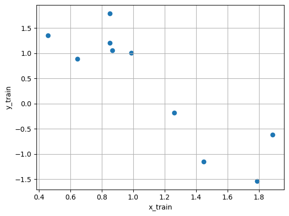
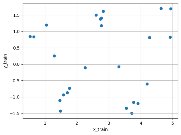
学習データの可視化
plt.figure(figsize=(10, 4))
plt.subplot(1, 2, 1)
plt.scatter(x_train, y_train, alpha=0.7)
plt.xlabel('x_train')
plt.ylabel('y_train')
plt.title('Training Data')
plt.grid(True)
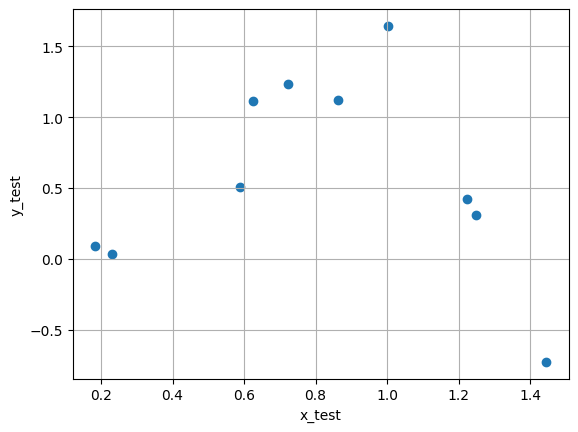
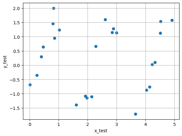
plt.subplot(1, 2, 2)
plt.scatter(x_test, y_test, alpha=0.7)
plt.xlabel('x_test')
plt.ylabel('y_test')
plt.title('Test Data')
plt.grid(True)
plt.tight_layout()
plt.show()
解空間次元Nの影響分析
# 異なるNに対する性能評価
diff = []
result = []

for N in range(2, 30):
    lss_c, M, Q = lms(x_train, y_train, N, 0.1)

    # 学習データを用いてyを推定
    ys_train = np.polyval(lss_c, x_train)

    # 検証データを用いてyを推定
    ys_test = np.polyval(lss_c, x_test)

    # 平均二乗誤差の計算
    train_error = mean_squared_error(y_train, ys_train)
    test_error = mean_squared_error(y_test, ys_test)

    result.append([train_error, test_error])

# 結果の可視化
diff = DataFrame(data=result, columns=['Training', 'Test'],
                index=[n for n in range(2, 30)])

diff.plot(title='Mean Squared Error vs Model Complexity (N)')
plt.xlabel('N (Model Complexity)')
plt.ylabel('MSE')
plt.grid(True)
plt.legend()
plt.show()
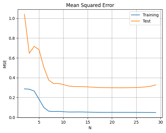
解空間次元の選択
- 低次元(N小):アンダーフィッティング、バイアスが大きい
- 高次元(N大):オーバーフィッティング、分散が大きい
- 適切な次元:バイアス-分散トレードオフの最適点
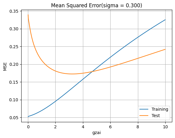
正則化パラメータξの最適化
N = 13
result = []

# 正則化パラメータの範囲を探索
for gzai_i in range(1, 1000):
    gzai = gzai_i * 0.01

    lss_c, M, Q = lms(x_train, y_train, N, gzai)

    # 予測値の計算
    ys_train = np.polyval(lss_c, x_train)
    ys_test = np.polyval(lss_c, x_test)

    # 誤差の計算
    train_error = mean_squared_error(y_train, ys_train)
    test_error = mean_squared_error(y_test, ys_test)

    result.append([gzai, train_error, test_error])

# 結果の可視化
diff = DataFrame(data=result, columns=['gzai', 'Training', 'Test'])

diff.plot(x='gzai', y=['Training', 'Test'])
plt.title(f'Mean Squared Error vs Regularization Parameter (σ = {sigma:.3f})')
plt.xlabel('ξ (Regularization Parameter)')
plt.ylabel('MSE')
plt.grid(True)
plt.show()
最適パラメータでの結果
N = 13
gzai = 0.32

lss_c, M, Q = lms(x_train, y_train, N, gzai)

# 予測曲線の生成
xs = np.linspace(np.min(x_train), np.max(x_train), M)
ys = np.polyval(lss_c, xs)

# 学習データの予測
ys_train = np.polyval(lss_c, x_train)

# 真の曲線
linex = np.arange(0, 2.0, 0.01)
liney = np.sin(np.pi*linex) - np.cos(np.pi*linex)

# 可視化
plt.figure(figsize=(10, 6))
plt.plot(linex, liney, color='green', linewidth=2, label='True Function')
plt.scatter(x_train, y_train, alpha=0.7, label='Training Data')
plt.plot(xs, ys, 'r-', lw=2, label='Regularized Fit')

plt.title(f'N = {N}, M = {M}, ξ = {gzai:.3f}')
plt.xlabel('x')
plt.ylabel('y')
plt.legend(loc='best', frameon=False)
plt.grid(True)
plt.show()

# 性能評価
ys_test = np.polyval(lss_c, x_test)

print(f'MSE (Training): {mean_squared_error(y_train, ys_train):.6f}')
print(f'MSE (Test): {mean_squared_error(y_test, ys_test):.6f}')
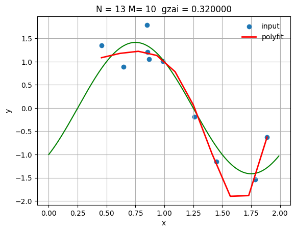
MSE (Training): 0.056731
MSE (Test): 0.268689
正則化の効果
適切な正則化パラメータを選択することで:
- 学習誤差とテスト誤差のバランスが取れる
- 過学習を防ぎ、汎化性能が向上する
- 数値的安定性が向上する
実験2:より複雑な関数近似
より大きなデータセットでの実験
設定:
- サンプル数:50(学習・テスト各25)
- 元の関数:
- ノイズ:平均0、標準偏差0.3の正規分布
sample = 50
sigma = 0.3

# ノイズ生成
e = np.random.normal(0, sigma, sample)

# より広い範囲での信号生成
x = np.random.uniform(0, 5, sample)
y = np.sin(np.pi*x) - np.cos(np.pi*x) + e

# データ分割
x_train, x_test, y_train, y_test = train_test_split(
    x, y, train_size=0.5, test_size=0.5, random_state=0
)
データの可視化
plt.figure(figsize=(12, 4))

plt.subplot(1, 2, 1)
plt.scatter(x_train, y_train, alpha=0.7)
plt.xlabel('x_train')
plt.ylabel('y_train')
plt.title('Training Data (Extended Range)')
plt.grid(True)

plt.subplot(1, 2, 2)
plt.scatter(x_test, y_test, alpha=0.7)
plt.xlabel('x_test')
plt.ylabel('y_test')
plt.title('Test Data (Extended Range)')
plt.grid(True)

plt.tight_layout()
plt.show()
解空間次元の影響(拡張版)
result = []

for N in range(2, 13):
    lss_c, M, Q = lms(x_train, y_train, N, 0.1)

    # 予測値計算
    ys_train = np.polyval(lss_c, x_train)
    ys_test = np.polyval(lss_c, x_test)

    # 誤差計算
    train_error = mean_squared_error(y_train, ys_train)
    test_error = mean_squared_error(y_test, ys_test)

    result.append([train_error, test_error])

# 結果可視化
diff = DataFrame(data=result, columns=['Training', 'Test'],
                index=[n for n in range(2, 13)])

diff.plot(title=f'M = {M}, ξ = 0.1: Mean Squared Error')
plt.xlabel('N (Model Complexity)')
plt.ylabel('MSE')
plt.grid(True)
plt.show()
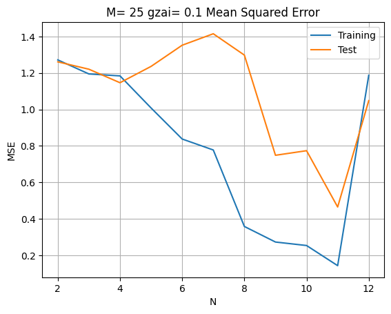
高次元での不安定性
の場合、 で誤差が急激に増加します。これは基底関数 が の範囲が大きいときに指数的に増加するためです。
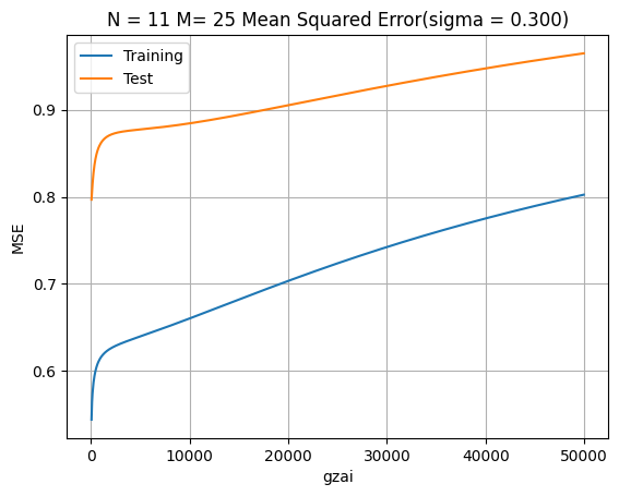
正則化パラメータの再調整
N = 11
result = []

# より大きな正則化パラメータの範囲を探索
for gzai_i in range(1, 1000):
    gzai = gzai_i * 50  # より大きな値を試行

    lss_c, M, Q = lms(x_train, y_train, N, gzai)

    # 予測と誤差計算
    ys_train = np.polyval(lss_c, x_train)
    ys_test = np.polyval(lss_c, x_test)

    train_error = mean_squared_error(y_train, ys_train)
    test_error = mean_squared_error(y_test, ys_test)

    result.append([gzai, train_error, test_error])

# 結果可視化
diff = DataFrame(data=result, columns=['gzai', 'Training', 'Test'])

diff.plot(x='gzai', y=['Training', 'Test'])
plt.title(f'N = {N}, M = {M}: Mean Squared Error (σ = {sigma:.3f})')
plt.xlabel('ξ (Regularization Parameter)')
plt.ylabel('MSE')
plt.grid(True)
plt.show()
小さな正則化パラメータでの結果
N = 11
gzai = 0.02

lss_c, M, Q = lms(x_train, y_train, N, gzai)

# 予測曲線生成
xs = np.linspace(np.min(x_train), np.max(x_train), M)
ys = np.polyval(lss_c, xs)

# 学習データ予測
ys_train = np.polyval(lss_c, x_train)

# 真の曲線
linex = np.arange(0, 5.0, 0.01)
liney = np.sin(np.pi*linex) - np.cos(np.pi*linex)

# 可視化
plt.figure(figsize=(12, 6))
plt.plot(linex, liney, color='green', linewidth=2, label='True Function')
plt.scatter(x_train, y_train, alpha=0.7, label='Training Data')
plt.plot(xs, ys, 'r-', lw=2, label='Regularized Fit')

plt.title(f'N = {N}, M = {M}, ξ = {gzai:.3f}')
plt.xlabel('x')
plt.ylabel('y')
plt.legend(loc='best', frameon=False)
plt.grid(True)
plt.show()

# 性能評価
ys_test = np.polyval(lss_c, x_test)

print(f'MSE (Training): {mean_squared_error(y_train, ys_train):.6f}')
print(f'MSE (Test): {mean_squared_error(y_test, ys_test):.6f}')
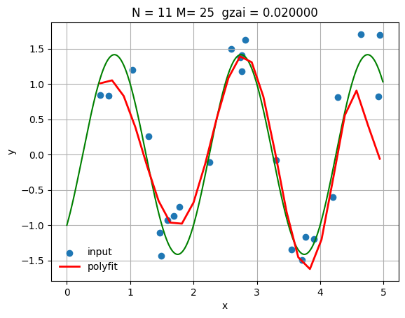
MSE (Training): 0.301408
MSE (Test): 0.335157
大きな正則化パラメータでの結果
N = 11
gzai = 10000

lss_c, M, Q = lms(x_train, y_train, N, gzai)

# 同様の可視化と評価
xs = np.linspace(np.min(x_train), np.max(x_train), M)
ys = np.polyval(lss_c, xs)
ys_train = np.polyval(lss_c, x_train)

linex = np.arange(0, 5.0, 0.01)
liney = np.sin(np.pi*linex) - np.cos(np.pi*linex)

plt.figure(figsize=(12, 6))
plt.plot(linex, liney, color='green', linewidth=2, label='True Function')
plt.scatter(x_train, y_train, alpha=0.7, label='Training Data')
plt.plot(xs, ys, 'r-', lw=2, label='Regularized Fit')

plt.title(f'N = {N}, M = {M}, ξ = {gzai:.0f}')
plt.xlabel('x')
plt.ylabel('y')
plt.legend(loc='best', frameon=False)
plt.grid(True)
plt.show()

ys_test = np.polyval(lss_c, x_test)

print(f'MSE (Training): {mean_squared_error(y_train, ys_train):.6f}')
print(f'MSE (Test): {mean_squared_error(y_test, ys_test):.6f}')
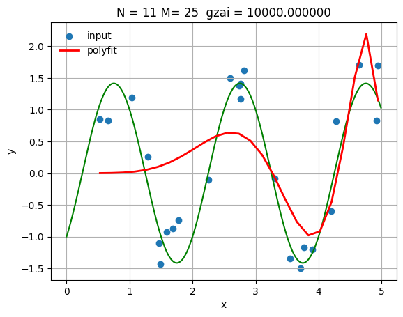
MSE (Training): 0.660348
MSE (Test): 0.884474
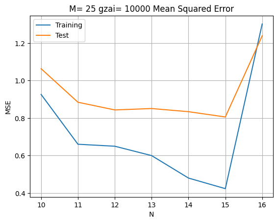
高次元での正則化効果
# 高次元モデルでの正則化効果を確認
result = []

for N in range(10, 17):
    lss_c, M, Q = lms(x_train, y_train, N, 10000)

    ys_train = np.polyval(lss_c, x_train)
    ys_test = np.polyval(lss_c, x_test)

    train_error = mean_squared_error(y_train, ys_train)
    test_error = mean_squared_error(y_test, ys_test)

    result.append([train_error, test_error])

diff = DataFrame(data=result, columns=['Training', 'Test'],
                index=[n for n in range(10, 17)])

diff.plot(title=f'M = {M}, ξ = 10000: Mean Squared Error')
plt.xlabel('N (Model Complexity)')
plt.ylabel('MSE')
plt.grid(True)
plt.show()
より高次元での最適化例
N = 15
gzai = 10000

lss_c, M, Q = lms(x_train, y_train, N, gzai)

xs = np.linspace(np.min(x_train), np.max(x_train), M)
ys = np.polyval(lss_c, xs)
ys_train = np.polyval(lss_c, x_train)

# 真の曲線
linex = np.arange(0, 5.0, 0.01)
liney = np.sin(np.pi*linex) - np.cos(np.pi*linex)

plt.figure(figsize=(12, 6))
plt.plot(linex, liney, color='green', linewidth=2, label='True Function')
plt.scatter(x_train, y_train, alpha=0.7, label='Training Data')
plt.plot(xs, ys, 'r-', lw=2, label='Regularized Fit')

plt.title(f'N = {N}, M = {M}, ξ = {gzai:.0f}')
plt.xlabel('x')
plt.ylabel('y')
plt.legend(loc='best', frameon=False)
plt.grid(True)
plt.show()

ys_test = np.polyval(lss_c, x_test)

print(f'MSE (Training): {mean_squared_error(y_train, ys_train):.6f}')
print(f'MSE (Test): {mean_squared_error(y_test, ys_test):.6f}')
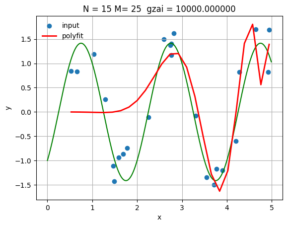
MSE (Training): 0.423424
MSE (Test): 0.805849
総合的な考察
1. モデル複雑さと正則化の関係
実験結果から、以下の重要な知見が得られました:
解空間次元 の効果:
- が大きいほど、モデルの表現能力が向上
- しかし、適切な正則化なしでは過学習のリスクが増大
- 基底関数 の特性により、 の範囲が大きい場合は特に注意が必要
正則化パラメータ の効果:
- 小さい値:学習誤差は小さいが、テスト誤差が大きい(過学習)
- 大きい値:安定した予測だが、アンダーフィッティングのリスク
- 最適値:バイアス-分散トレードオフの最適化
2. 実用的な指針
モデル選択戦略:
- クロスバリデーション:正則化パラメータの選択
- 情報量規準:AICやBICによるモデル比較
- 早期停止:反復的手法での過学習防止
基底関数の設計:
- 入力データの範囲に適した基底関数の選択
- 直交基底(チェビシェフ多項式など)の使用を検討
- スプライン基底や動径基底関数の活用
3. 数値的安定性
計算上の注意点:
- 条件数の監視:
- SVD分解の活用:数値的により安定な実装
- 適応的正則化:データに応じた動的調整
実用的な拡張
- リッジ回帰(L2正則化):本手法の標準的な名称
- ラッソ回帰(L1正則化):スパース解を得る手法
- エラスティックネット:L1とL2の組み合わせ
- ベイズ的解釈:正則化項を事前分布として解釈
まとめ
正則化ミニマムノルム解は、線形回帰における重要な手法であり、以下の特徴を持ちます:
- 過学習の防止:正則化項により汎化性能を向上
- 数値的安定性:特異値問題の回避
- 柔軟なモデル選択:パラメータ調整による複雑さ制御
適切な正則化パラメータとモデル複雑さの選択により、実用的で堅牢な予測モデルを構築できます。現代の機械学習において、正則化は必須の技術となっており、深層学習を含む様々な手法の基礎となっています。
次のステップ
- カーネル法:非線形関数近似への拡張
- ガウス過程回帰:不確実性の定量化
- ベイズ線形回帰:確率的な解釈
- スパース回帰:特徴選択を含む手法