正則化ミニマムノルム解(Regularized minimal-norm solution)
Home Page:Youkoutaku
1
2
3
4
5
6
7
8
9
10
11
12
13
14
15
16
17
import numpy as np
import scipy as sp
import pandas as pd
from pandas import Series, DataFrame
from sklearn.metrics import mean_squared_error

import matplotlib.pyplot as plt
import matplotlib as mpl
import seaborn as sns
%matplotlib inline

# 小数第3位まで表示
%precision 3

# ランダムシードの固定
np.random.seed(123)
正則化ミニマムノルム解関数
1
2
3
4
5
6
7
8
9
10
11
12
13
14
15
16
17
18
19
20
21
22
23
24
25
26
27
28
29
30
31
# 正則化ミニマムノルム解を求める rmls(学習データx(x_train), 学習データy(y_train), 解空間の次元数N, 正規化定数ξ)
def lms(x_train, y_train, N, gzai ):

    #行列Hの行数設定
    M=x_train.shape[0]

    #xとyをM行1列に変換
    x_train=x_train.reshape((M,1))
    y_train=y_train.reshape((M,1))

    #全ての要素が1の列ベクトルを生成
    i=np.ones((M,1))

    H=i
    for k in range(1,N):
        H=np.hstack((H,x_train**k))
    #print('H =', H)


    #パラメータΘの最小二乗推定値
    A=np.dot(H, H.T)+gzai*np.eye(M)

    lss_c=np.dot(np.dot(H.T,np.linalg.inv(A)),y_train)

    #分解能行列Qの計算
    Q=np.dot(np.dot(H.T,np.linalg.inv(A)),H)

    #lss_cの要素を逆順に並び替え
    lss_c=np.sort(lss_c)[::-1]

    return (lss_c, M, Q)
関数1
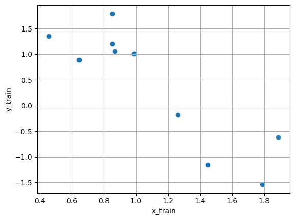
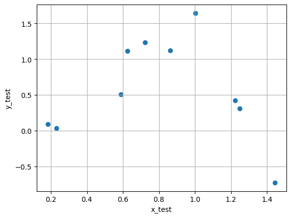
観測データの生成
サンプル:$20$(学習とテストデータを分けることで,観測空間M=10)
元の関数:
\[y=sin(x)+cos(x), 0<x<2\]ノイズ: 平均0,標準偏差0.3の正規分布
1
2
3
4
5
6
7
8
9
10
11
12
13
14
15
16
17
18
19
20
21
x = []
y = []
#サンプル数
sample = 20
#ノイズ標準偏差
sigma=0.3

# ノイズ(正規分布)
# np.random.normal(平均、標準偏差、サンプル数)
e= np.random.normal(0, sigma, sample)
#eo= np.random.normal(0, sigma, m)


# 信号生成
#np.random.uniform(a, b, サンプル数) aからbまでの一様乱数
x=np.random.uniform(0, 2, sample)
y = np.sin(np.pi*x) - np.cos(np.pi*x)  + e

# データを学習用と検証用に分割
from sklearn.model_selection import train_test_split
x_train, x_test, y_train, y_test = train_test_split(x, y, train_size = 0.5, test_size = 0.5, random_state = 0)
1
2
3
4
plt.scatter(x_train, y_train)
plt.xlabel('x_train')
plt.ylabel('y_train')
plt.grid(True)
1
2
3
4
plt.scatter(x_test, y_test)
plt.xlabel('x_test')
plt.ylabel('y_test')
plt.grid(True)
解空間Nの考察
1
2
3
4
5
6
7
8
9
10
11
12
13
14
15
16
17
18
19
20
diff = []
result= []
for N in range(2,30):
  lss_c, M, Q = lms(x_train, y_train, N, 0.1)
 #学習データを用いてyを推定
  ys_train= np.polyval(lss_c,x_train)
 #検証データを用いてyを推定
  ys_test=np.polyval(lss_c,x_test)
 #学習データに対するyの推定値の平均二乗誤差
  train_error= mean_squared_error(y_train, ys_train)
 #検証データに対するyの推定値の平均二乗誤差
  test_error= mean_squared_error(y_test, ys_test)
  result.append([train_error, test_error])

diff = DataFrame(data=result, columns=['Training','Test'], index=[n for n in range(2,30)])

diff.plot(title='Mean Squared Error')
plt.xlabel('N')
plt.ylabel('MSE')
plt.grid(True)
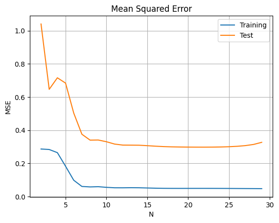
これにより,解空間Nが大きくなると,推定精度が上がる。
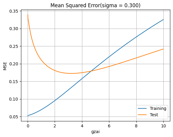
正則化パラメータ$\xi$の考察
1
2
3
4
5
6
7
8
9
10
11
12
13
14
15
16
17
18
19
20
21
22
23
24
25
26
27
28
29
30
31
32
33
N=13
#学習データと検証データでの平均二乗誤差(MSE)の表示
result=[]
#diff = DataFrame(columns=['gzai','Training','Test'])
for gzai_i in range(1,1000):

    gzai=gzai_i*0.01

    lss_c, M, Q = lms(x_train, y_train,  N, gzai)

    #学習データを用いてyを推定
    ys_train = np.polyval(lss_c,x_train)

    #検証データを用いてyを推定
    ys_test=np.polyval(lss_c,x_test)

    #学習データに対するyの推定の平均二乗誤差
    train_error = mean_squared_error(y_train, ys_train)

    #検証データに対するyの推定の平均二乗誤差
    test_error = mean_squared_error(y_test, ys_test)

    result.append([gzai, train_error, test_error])

diff = DataFrame(data=result, columns=['gzai','Training','Test'])

#回帰モデルの性能評価の結果表示
diff.plot(x='gzai', y=['Training', 'Test'])

plt.title('Mean Squared Error(sigma = %.3f)' % (sigma))
plt.xlabel('gzai')
plt.ylabel('MSE')
plt.grid(True)
1
2
3
4
5
6
7
8
9
10
11
12
13
14
15
16
17
18
19
20
21
22
23
24
25
26
27
28
29
30
31
32
33
34
35
36
37
N = 13
gzai=0.32

lss_c, M, Q =lms(x_train, y_train, N, gzai)

xs = np.linspace(np.min(x_train),np.max(x_train),M)
ys = np.polyval(lss_c,xs)

#学習データを用いてyを推定
ys_train = np.polyval(lss_c,x_train)

# 真の曲線を表示
linex = np.arange(0, 2.0, 0.01)
liney = np.sin(np.pi*linex) - np.cos(np.pi*linex)
plt.plot(linex, liney, color='green')

plt.scatter(x_train, y_train,label='input')
plt.plot(xs, ys, 'r-', lw=2, label='polyfit')


plt.title('N = %d M= %d  gzai = %f' % (N, M, gzai))
plt.xlabel('x')
plt.ylabel('y')
plt.legend(loc='best',frameon=False)
plt.grid(True)

#回帰モデルの性能評価(平均二乗誤差)
from sklearn.metrics import mean_squared_error

#検証データを用いてyを推定
ys_test=np.polyval(lss_c,x_test)

#学習データに対するyの推定の平均二乗誤差
print('MSE train data: ', mean_squared_error(y_train, ys_train))

#検証データに対するyの推定の平均二乗誤差
print('MSE test data: ', mean_squared_error(y_test, ys_test))
1
2
MSE train data:  0.056731303121826726
MSE test data:  0.2686888238391384
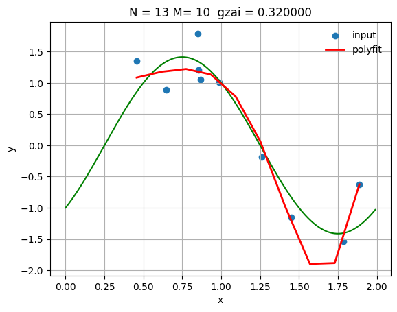
これによって,正則化パラメータを適切に選択することで,学習効果とテスト結果に影響がある。
関数2
観測データの生成
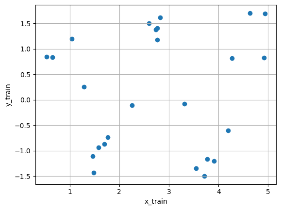
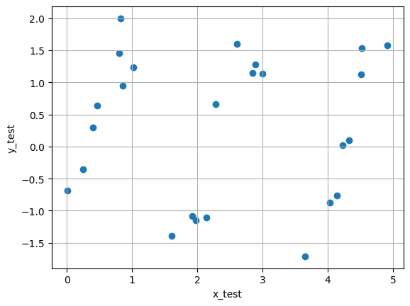
サンプル:50(学習とテストデータを分けることで,観測空間M=25)
元の関数: \(y=sin(x)+cos(x), 0<x<5\)
ノイズ: 平均0,標準偏差0.3の正規分布
1
2
3
4
5
6
7
8
9
10
11
12
13
14
15
16
17
18
sample = 50
#ノイズ標準偏差
sigma=0.3

# ノイズ(正規分布)
# np.random.normal(平均、標準偏差、サンプル数)
e= np.random.normal(0, sigma, sample)
#eo= np.random.normal(0, sigma, m)


# 信号生成
#np.random.uniform(a, b, サンプル数) aからbまでの一様乱数
x=np.random.uniform(0, 5, sample)
y = np.sin(np.pi*x) - np.cos(np.pi*x)  + e

# データを学習用と検証用に分割
from sklearn.model_selection import train_test_split
x_train, x_test, y_train, y_test = train_test_split(x, y, train_size = 0.5, test_size = 0.5, random_state = 0)
1
2
3
4
plt.scatter(x_train, y_train)
plt.xlabel('x_train')
plt.ylabel('y_train')
plt.grid(True)
1
2
3
4
plt.scatter(x_test, y_test)
plt.xlabel('x_test')
plt.ylabel('y_test')
plt.grid(True)
解空間$N$の考察
1
2
3
4
5
6
7
8
9
10
11
12
13
14
15
16
17
18
19
20
21
22
23
lss_c=[]
M =[]
Q = []
diff =[]
result=[]
for N in range(2,13):
  lss_c, M, Q = lms(x_train, y_train, N, 0.1)
 #学習データを用いてyを推定
  ys_train= np.polyval(lss_c,x_train)
 #検証データを用いてyを推定
  ys_test=np.polyval(lss_c,x_test)
 #学習データに対するyの推定値の平均二乗誤差
  train_error= mean_squared_error(y_train, ys_train)
 #検証データに対するyの推定値の平均二乗誤差
  test_error= mean_squared_error(y_test, ys_test)
  result.append([train_error, test_error])

diff = DataFrame(data=result, columns=['Training','Test'], index=[n for n in range(2,13)])

diff.plot(title='M= %d gzai= 0.1 Mean Squared Error' % (M))
plt.xlabel('N')
plt.ylabel('MSE')
plt.grid(True)
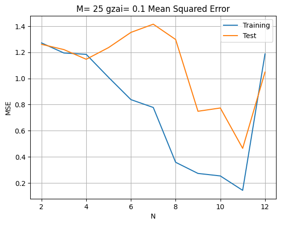
ここで$\xi=0.1$の場合,$N>11$にすると,誤差が逆に大きくなる。その理由について,正則化パラメータ$\xi$が適切ではないと考えるために,以下のように考察を行った。
正則化パラメータ$\xi$の考察
1
2
3
4
5
6
7
8
9
10
11
12
13
14
15
16
17
18
19
20
21
22
23
24
25
26
27
28
29
30
31
32
33
#学習データと検証データでの平均二乗誤差(MSE)の表示
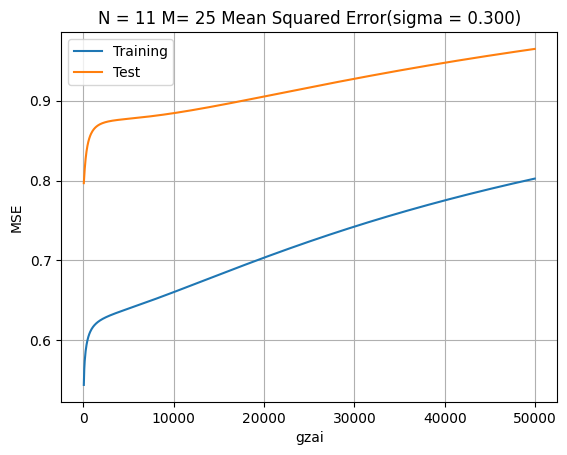
N=11
result=[]
#diff = DataFrame(columns=['gzai','Training','Test'])
for gzai_i in range(1,1000):
gzai=gzai_i*50
lss_c, M, Q = lms(x_train, y_train, N, gzai)
#学習データを用いてyを推定
ys_train = np.polyval(lss_c,x_train)
#検証データを用いてyを推定
ys_test=np.polyval(lss_c,x_test)
#学習データに対するyの推定の平均二乗誤差
train_error = mean_squared_error(y_train, ys_train)
#検証データに対するyの推定の平均二乗誤差
test_error = mean_squared_error(y_test, ys_test)
result.append([gzai, train_error, test_error])
diff = DataFrame(data=result, columns=['gzai','Training','Test'])
#回帰モデルの性能評価の結果表示
diff.plot(x='gzai', y=['Training', 'Test'])
plt.title('N = %d M= %d Mean Squared Error(sigma = %.3f)' % (N, M, sigma))
plt.xlabel('gzai')
plt.ylabel('MSE')
plt.grid(True)
1
2
3
4
5
6
7
8
9
10
11
12
13
14
15
16
17
18
19
20
21
22
23
24
25
26
27
28
29
30
31
32
33
34
35
36
37
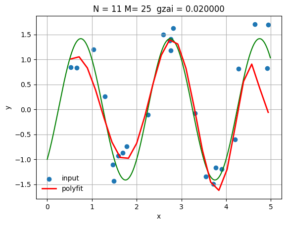
N = 11
gzai=0.02
lss_c, M, Q =lms(x_train, y_train, N, gzai)
xs = np.linspace(np.min(x_train),np.max(x_train),M)
ys = np.polyval(lss_c,xs)
#学習データを用いてyを推定
ys_train = np.polyval(lss_c,x_train)
# 真の曲線を表示
linex = np.arange(0, 5.0, 0.01)
liney = np.sin(np.pi*linex) - np.cos(np.pi*linex)
plt.plot(linex, liney, color='green')
plt.scatter(x_train, y_train,label='input')
plt.plot(xs, ys, 'r-', lw=2, label='polyfit')
plt.title('N = %d M= %d gzai = %f' % (N, M, gzai))
plt.xlabel('x')
plt.ylabel('y')
plt.legend(loc='best',frameon=False)
plt.grid(True)
#回帰モデルの性能評価(平均二乗誤差)
from sklearn.metrics import mean_squared_error
#検証データを用いてyを推定
ys_test=np.polyval(lss_c,x_test)
#学習データに対するyの推定の平均二乗誤差
print('MSE train data: ', mean_squared_error(y_train, ys_train))
#検証データに対するyの推定の平均二乗誤差
print('MSE test data: ', mean_squared_error(y_test, ys_test))
1
2
MSE train data:  0.3014076921109078
MSE test data:  0.3351574787240519
1
2
3
4
5
6
7
8
9
10
11
12
13
14
15
16
17
18
19
20
21
22
23
24
25
26
27
28
29
30
31
32
33
34
35
36
37
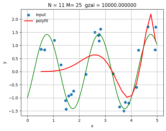
N = 11
gzai=10000
lss_c, M, Q =lms(x_train, y_train, N, gzai)
xs = np.linspace(np.min(x_train),np.max(x_train),M)
ys = np.polyval(lss_c,xs)
#学習データを用いてyを推定
ys_train = np.polyval(lss_c,x_train)
# 真の曲線を表示
linex = np.arange(0, 5.0, 0.01)
liney = np.sin(np.pi*linex) - np.cos(np.pi*linex)
plt.plot(linex, liney, color='green')
plt.scatter(x_train, y_train,label='input')
plt.plot(xs, ys, 'r-', lw=2, label='polyfit')
plt.title('N = %d M= %d gzai = %f' % (N, M, gzai))
plt.xlabel('x')
plt.ylabel('y')
plt.legend(loc='best',frameon=False)
plt.grid(True)
#回帰モデルの性能評価(平均二乗誤差)
from sklearn.metrics import mean_squared_error
#検証データを用いてyを推定
ys_test=np.polyval(lss_c,x_test)
#学習データに対するyの推定の平均二乗誤差
print('MSE train data: ', mean_squared_error(y_train, ys_train))
#検証データに対するyの推定の平均二乗誤差
print('MSE test data: ', mean_squared_error(y_test, ys_test))
1
2
MSE train data:  0.6603476532318381
MSE test data:  0.8844738123048232
1
2
3
4
5
6
7
8
9
10
11
12
13
14
15
16
17
18
19
result=[]
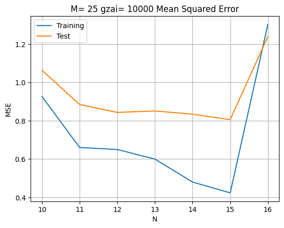
for N in range(10,17):
lss_c, M, Q = lms(x_train, y_train, N, 10000)
#学習データを用いてyを推定
ys_train= np.polyval(lss_c,x_train)
#検証データを用いてyを推定
ys_test=np.polyval(lss_c,x_test)
#学習データに対するyの推定値の平均二乗誤差
train_error= mean_squared_error(y_train, ys_train)
#検証データに対するyの推定値の平均二乗誤差
test_error= mean_squared_error(y_test, ys_test)
result.append([train_error, test_error])
diff = DataFrame(data=result, columns=['Training','Test'], index=[n for n in range(10,17)])
diff.plot(title='M= %d gzai= 10000 Mean Squared Error' % (M))
plt.xlabel('N')
plt.ylabel('MSE')
plt.grid(True)
$N=11$の場合で,$\xi$を考察することで,正則化パラメータが非常に小さい時(0.1),学習効果がとても良いことが分かった。しかし,この時にはテスト結果は最適ではない。正則化パラメータの増加とともに,テスト結果がよくなるが,学習効果が低下している。
1
2
3
4
5
6
7
8
9
10
11
12
13
14
15
16
17
18
19
20
21
22
23
24
25
26
27
28
29
30
31
32
33
34
35
36
37
N = 15
gzai=10000

lss_c, M, Q =lms(x_train, y_train, N, gzai)

xs = np.linspace(np.min(x_train),np.max(x_train),M)
ys = np.polyval(lss_c,xs)

#学習データを用いてyを推定
ys_train = np.polyval(lss_c,x_train)

# 真の曲線を表示
linex = np.arange(0, 5.0, 0.01)
liney = np.sin(np.pi*linex)- np.cos(np.pi*linex)
plt.plot(linex, liney, color='green')

plt.scatter(x_train, y_train,label='input')
plt.plot(xs, ys, 'r-', lw=2, label='polyfit')


plt.title('N = %d M= %d  gzai = %f' % (N, M, gzai))
plt.xlabel('x')
plt.ylabel('y')
plt.legend(loc='best',frameon=False)
plt.grid(True)

#回帰モデルの性能評価(平均二乗誤差)
from sklearn.metrics import mean_squared_error

#検証データを用いてyを推定
ys_test=np.polyval(lss_c,x_test)

#学習データに対するyの推定の平均二乗誤差
print('MSE train data: ', mean_squared_error(y_train, ys_train))

#検証データに対するyの推定の平均二乗誤差
print('MSE test data: ', mean_squared_error(y_test, ys_test))
1
2
MSE train data:  0.42342416627062157
MSE test data:  0.8058493745194096
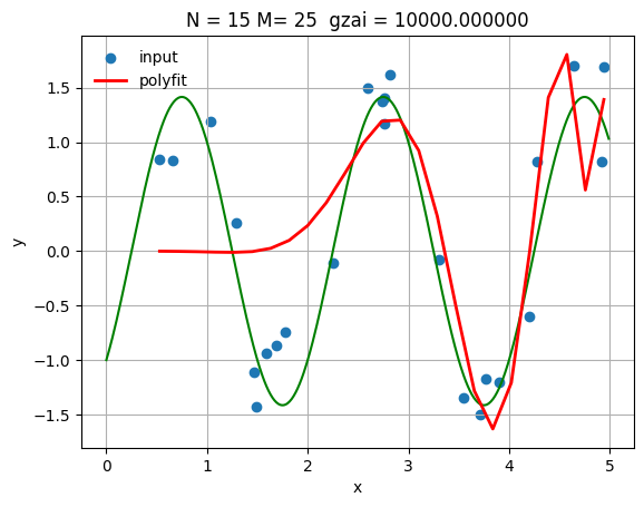
これによって,正則化パラメータが大きくすると,$N>11$でも誤差が普通になる。
考察
したがって,以下のような考察結果が得られる。
- 解空間$N$が大きいほど線形回帰の正則化ミニマムノルム解がよくなる。また,正則化パラメータ $\xi$ が小さくすると,学習効果が良くなる。正則化パラメータ $\xi$ が大きくなると,学習効果が悪くなるが,テスト結果がよくなる。
- 解空間$N$が大きい場合に逆に効果が非常に悪くなることもある。また,正則化パラメータが前述と同じ効果がある。ただし,大きな解空間$N$を合わせるために適切な非常に大きい正則化パラメータを選択するすれば,良い結果が得られる。
しかし,今回のプログラムは,解く関数lms()学習データの数を観測空間$M$としている。
M=x_train.shape[0]
これはあくまでも学習データのサンプル数であり,信号関数が実際には非線形関数である。関数1では$0<x<2$に対して,$サンプルM=10$を取った。関数2では$0<x<5$に対して,$サンプルM=25$を取った。 サンプリング周期の定理を考えてもサンプリング周期が同じである。
乱数数列の影響を考えずに,このような問題が生じるのは,基底関数が$\phi_x(k)=x^k$設計されるために,$x$の範囲が大きい場合,解空間$N$が大きいほど基底関数が指数的に増加するため,推定効果が悪くなり,誤差が非常に大きくなる。
結論
- モデルの複雑さ 𝑁 を選択する時に,観測空間$M$を比べて大きいほどモデルの性能が良くなるが,設計した基底関数 $\phi_x(k)$を考慮する必要がある。 2.正則化パラメータ 𝜉 は過剰学習を防ぐために使用されるが、過度に大きすぎるとモデルの性能が低下する可能性があるため、適切な値を選択することが重要である。