Made by Youkoutaku
1
2
3
4
| # Library Import
import numpy as np
import matplotlib.pyplot as plt
from scipy.stats import bernoulli, binom, geom, nbinom, poisson, hypergeom, uniform, norm, expon, gamma, chi2
|
- 離散分布
bernouli: ベルヌーイ分布binom: 2項分布geom: 幾何分布nbinom: 負の2項分布poisson: ポアソン分布hypergeom: 超幾何分布
- 連続分布
uniform: 一様分布norm: 正規分布gamma: ガンマ分布chi2: カイ二乗分布
- Method
rvs: 確率変数pmf: 確率関数(離散)pbf: 確率密度関数(連続)
1.離散確率分布
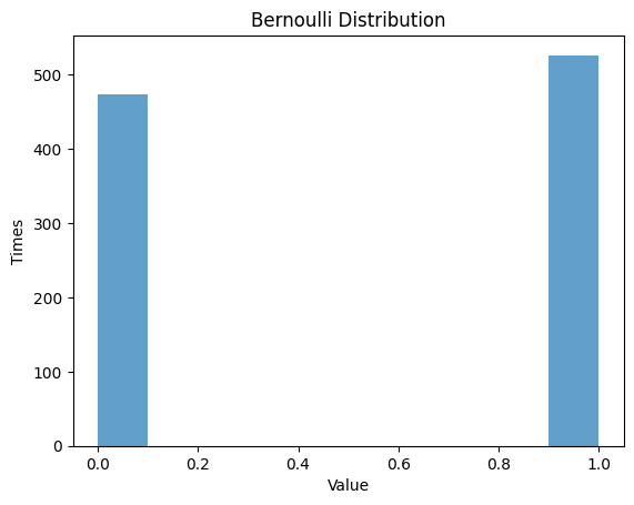
1.1 ベルヌーイ分布
- ベルヌーイ分布は、1回の試行で成功または失敗の2つの結果しかない離散確率分布です。
- 確率パラメータ $p$ を設定し、それに従う疑似乱数列を生成します。
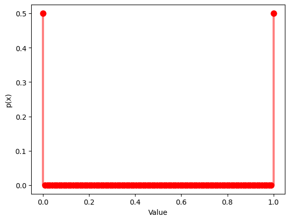
1.1.1 $p$ $=0.5$
疑似乱数数列での分布関数と確率関数:
1
2
3
4
5
6
7
8
9
10
11
12
13
14
15
16
17
18
19
| p = 0.5 # Probability
rv_bernoulli = bernoulli(p)
data_bernoulli = rv_bernoulli.rvs(size=1000) # size=1000
# Randm Variable
plt.hist(data_bernoulli, alpha=0.7)
plt.title('Bernoulli Distribution')
plt.xlabel('Value')
plt.ylabel('Times')
plt.show()
# Probability mass function
x = np.linspace(0, 1, 100)
y = bernoulli.pmf(x, p)
plt.plot(x, y, 'ro', ms=8)
plt.vlines(x, 0, y, colors='r', lw=3, alpha=0.5)
plt.xlabel('Value')
plt.ylabel('p(x)')
plt.show()
|
特性値:
1
2
3
4
5
6
7
8
9
10
11
12
13
| theoretical_mean = p
theoretical_std = np.sqrt(p * (1 - p))
# Calculation of actual values
mean_bernoulli = np.mean(data_bernoulli)
std_bernoulli = np.std(data_bernoulli)
# Comparison of theoretical and measured values
print("Bernoulli Distribution:")
print("Theoretical Mean:", theoretical_mean)
print("Computed Mean:", mean_bernoulli)
print("Theoretical Standard Deviation:", theoretical_std)
print("Computed Standard Deviation:", std_bernoulli)
|
1
2
3
4
5
| Bernoulli Distribution:
Theoretical Mean: 0.5
Computed Mean: 0.526
Theoretical Standard Deviation: 0.5
Computed Standard Deviation: 0.4993235424051224
|
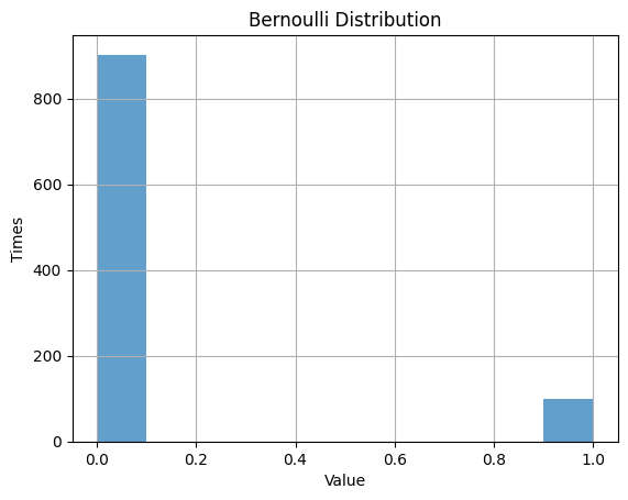
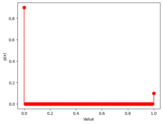
1.1.2 $p$ $= 0.1$
1
2
3
4
5
6
7
8
9
10
11
12
13
14
15
16
17
18
19
20
| p = 0.1 # probability
rv_bernoulli = bernoulli(p)
data_bernoulli = rv_bernoulli.rvs(size=1000) # size=1000
# Randm Variable
plt.hist(data_bernoulli, alpha=0.7)
plt.title('Bernoulli Distribution')
plt.xlabel('Value')
plt.ylabel('Times')
plt.grid(True)
plt.show()
# Probability mass function
x = np.linspace(0, 1, 100)
y = bernoulli.pmf(x, p)
plt.plot(x, y, 'ro', ms=8)
plt.vlines(x, 0, y, colors='r', lw=3, alpha=0.5)
plt.xlabel('Value')
plt.ylabel('p(x)')
plt.show()
|
特性値:
1
2
3
4
5
6
7
8
9
10
11
12
13
| theoretical_mean = p
theoretical_std = np.sqrt(p * (1 - p))
# Calculation of actual values
mean_bernoulli = np.mean(data_bernoulli)
std_bernoulli = np.std(data_bernoulli)
# Comparison of theoretical and measured values
print("Bernoulli Distribution:")
print("Theoretical Mean:", theoretical_mean)
print("Computed Mean:", mean_bernoulli)
print("Theoretical Standard Deviation:", theoretical_std)
print("Computed Standard Deviation:", std_bernoulli)
|
1
2
3
4
5
| Bernoulli Distribution:
Theoretical Mean: 0.1
Computed Mean: 0.098
Theoretical Standard Deviation: 0.30000000000000004
Computed Standard Deviation: 0.2973146481423342
|
観察:実測値の平均と標本誤差は理論値とほぼ同じである.
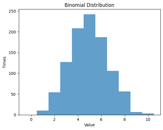
1.2 2項分布
- 2項分布は、独立したベルヌーイ試行を複数回行った場合の成功回数の確率分布です。
- 成功確率 $p$ と試行回数 $n$ の2つのパラメータを設定し、その分布を観察します。
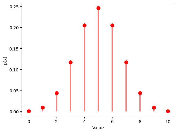
1.2.1 $p$ $=0.5$ , $n$ $=10$
1
2
3
4
5
6
7
8
9
10
11
12
13
14
15
16
17
18
19
20
21
| n = 10 # number of random experiments
p = 0.5 # probability
# Randm Variable
rv_binom = binom(n, p)
data_binom = rv_binom.rvs(size=1000)
plt.hist(data_binom, bins=np.arange(-0.5, n+1, 1), alpha=0.7)
plt.title('Binomial Distribution')
plt.xlabel('Value')
plt.ylabel('Times')
plt.show()
# Probability mass function
x = np.arange(0, 11)
y = binom.pmf(x, n, p)
plt.plot(x, y, 'ro', ms=8)
plt.vlines(x, 0, y, colors='r', lw=3, alpha=0.5)
plt.xlabel('Value')
plt.ylabel('p(x)')
plt.show()
|
1
2
3
4
5
6
7
8
9
10
| theoretical_mean_binom = n * p
theoretical_std_binom = np.sqrt(n * p * (1 - p))
mean_binom = np.mean(data_binom)
std_binom = np.std(data_binom)
print("\nBinomial Distribution:")
print("Theoretical Mean:", theoretical_mean_binom)
print("Computed Mean:", mean_binom)
print("Theoretical Standard Deviation:", theoretical_std_binom)
print("Computed Standard Deviation:", std_binom)
|
1
2
3
4
5
| Binomial Distribution:
Theoretical Mean: 5.0
Computed Mean: 4.946
Theoretical Standard Deviation: 1.5811388300841898
Computed Standard Deviation: 1.63128293070209
|
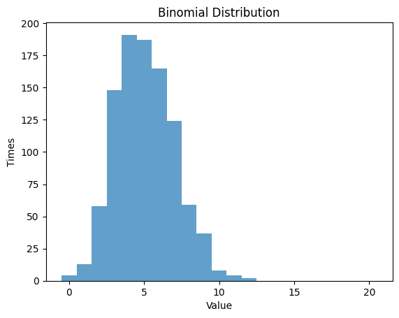
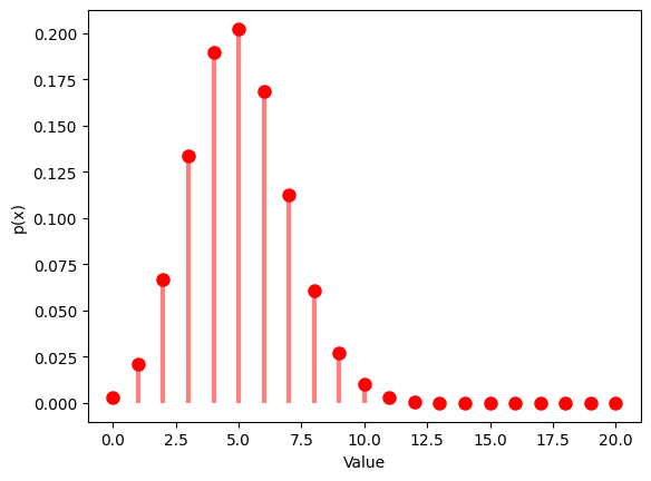
1.2.2 $p$ $=0.25$ , $n$ $=20$
1
2
3
4
5
6
7
8
9
10
11
12
13
14
15
16
17
18
19
20
| n = 20 # number of random experiments
p = 0.25 # probability
# Randm Variable
rv_binom = binom(n, p)
data_binom = rv_binom.rvs(size=1000)
plt.hist(data_binom, bins=np.arange(-0.5, n+1, 1), alpha=0.7)
plt.title('Binomial Distribution')
plt.xlabel('Value')
plt.ylabel('Times')
plt.show()
# Probability mass function
x = np.arange(0, 21)
y = binom.pmf(x, n, p)
plt.plot(x, y, 'ro', ms=8)
plt.vlines(x, 0, y, colors='r', lw=3, alpha=0.5)
plt.xlabel('Value')
plt.ylabel('p(x)')
plt.show()
|
1
2
3
4
5
6
7
8
9
10
| theoretical_mean_binom = n * p
theoretical_std_binom = np.sqrt(n * p * (1 - p))
mean_binom = np.mean(data_binom)
std_binom = np.std(data_binom)
print("\nBinomial Distribution:")
print("Theoretical Mean:", theoretical_mean_binom)
print("Computed Mean:", mean_binom)
print("Theoretical Standard Deviation:", theoretical_std_binom)
print("Computed Standard Deviation:", std_binom)
|
1
2
3
4
5
| Binomial Distribution:
Theoretical Mean: 5.0
Computed Mean: 5.083
Theoretical Standard Deviation: 1.9364916731037085
Computed Standard Deviation: 1.9575778400870807
|
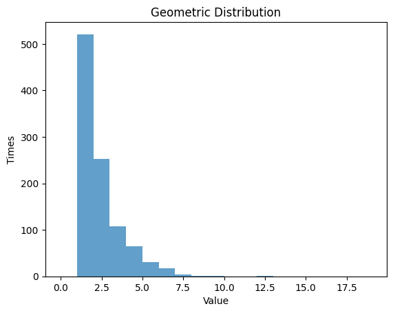
1.3 幾何分布
- 幾何分布は、最初の成功までの試行回数の確率分布です。
- 成功確率 $p$ を設定し、その分布を観察します。
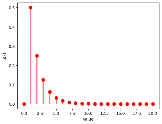
1.3.1 $p$ $=0.5$
1
2
3
4
5
6
7
8
9
10
11
12
13
14
15
16
17
18
19
| p = 0.5
rv_geom = geom(p)
data_geom = rv_geom.rvs(size=1000)
# Randm Variable
plt.hist(data_geom, bins=np.arange(0, 20, 1), alpha=0.7)
plt.title('Geometric Distribution')
plt.xlabel('Value')
plt.ylabel('Times')
plt.show()
# Probability mass function
x = np.arange(0, 21)
y = geom.pmf(x, p)
plt.plot(x, y, 'ro', ms=8)
plt.vlines(x, 0, y, colors='r', lw=3, alpha=0.5)
plt.xlabel('Value')
plt.ylabel('p(x)')
plt.show()
|
1
2
3
4
5
6
7
8
9
10
| theoretical_mean_geom = 1 / p
theoretical_std_geom = np.sqrt((1 - p) / (p ** 2))
mean_geom = np.mean(data_geom)
std_geom = np.std(data_geom)
print("\nGeometric Distribution:")
print("Theoretical Mean:", theoretical_mean_geom)
print("Computed Mean:", mean_geom)
print("Theoretical Standard Deviation:", theoretical_std_geom)
print("Computed Standard Deviation:", std_geom)
|
1
2
3
4
5
| Geometric Distribution:
Theoretical Mean: 2.0
Computed Mean: 1.922
Theoretical Standard Deviation: 1.4142135623730951
Computed Standard Deviation: 1.315262711400274
|
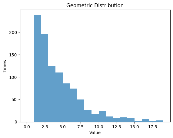
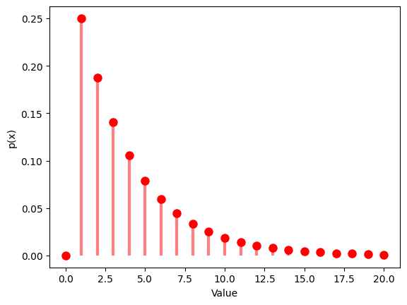
1.3.2 $p$ $=0.25$
1
2
3
4
5
6
7
8
9
10
11
12
13
14
15
16
17
18
19
| p = 0.25
rv_geom = geom(p)
data_geom = rv_geom.rvs(size=1000)
# Randm Variable
plt.hist(data_geom, bins=np.arange(0, 20, 1), alpha=0.7)
plt.title('Geometric Distribution')
plt.xlabel('Value')
plt.ylabel('Times')
plt.show()
# Probability mass function
x = np.arange(0, 21)
y = geom.pmf(x, p)
plt.plot(x, y, 'ro', ms=8)
plt.vlines(x, 0, y, colors='r', lw=3, alpha=0.5)
plt.xlabel('Value')
plt.ylabel('p(x)')
plt.show()
|
1
2
3
4
5
6
7
8
9
10
| theoretical_mean_geom = 1 / p
theoretical_std_geom = np.sqrt((1 - p) / (p ** 2))
mean_geom = np.mean(data_geom)
std_geom = np.std(data_geom)
print("\nGeometric Distribution:")
print("Theoretical Mean:", theoretical_mean_geom)
print("Computed Mean:", mean_geom)
print("Theoretical Standard Deviation:", theoretical_std_geom)
print("Computed Standard Deviation:", std_geom)
|
1
2
3
4
5
| Geometric Distribution:
Theoretical Mean: 4.0
Computed Mean: 4.027
Theoretical Standard Deviation: 3.4641016151377544
Computed Standard Deviation: 3.4023919527297264
|
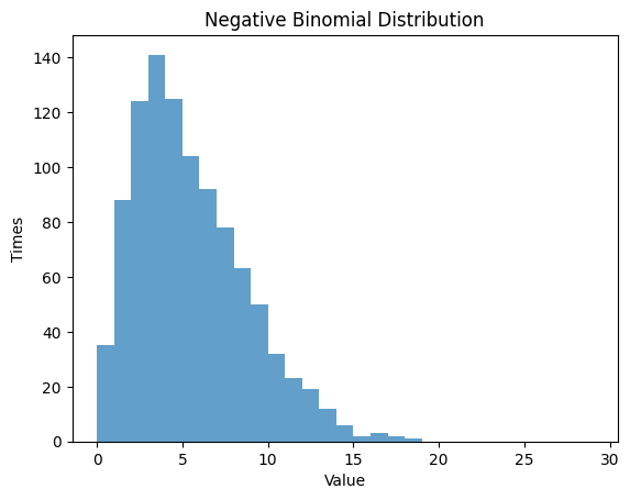
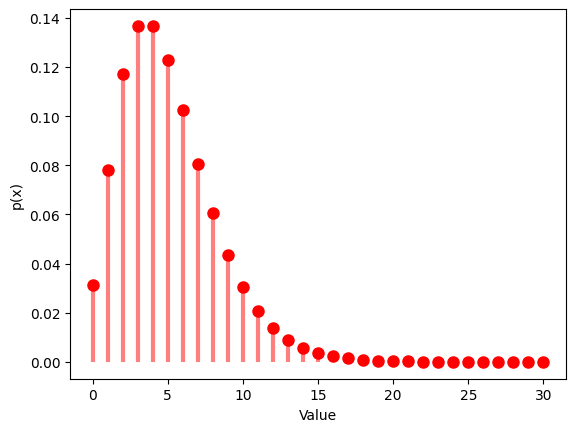
1.4 負の2項分布
- 負の2項分布は、成功回数が一定の値 $r$ に到達するまでのベルヌーイ試行の回数の確率分布です。
- 成功確率 $p$と成功回数 $r$ の2つのパラメータを設定し、その分布を観察します。
1.4.1 $p$ $=0.5$ , $n$ $=5$
1
2
3
4
5
6
7
8
9
10
11
12
13
14
15
16
17
18
19
20
| r = 5
p = 0.5
rv_nbinom = nbinom(r, p)
data_nbinom = rv_nbinom.rvs(size=1000)
# Randm Variable
plt.hist(data_nbinom, bins=np.arange(0, 30, 1), alpha=0.7)
plt.title('Negative Binomial Distribution')
plt.xlabel('Value')
plt.ylabel('Times')
plt.show()
# Probability mass function
x = np.arange(0, 31)
y = nbinom.pmf(x, r, p)
plt.plot(x, y, 'ro', ms=8)
plt.vlines(x, 0, y, colors='r', lw=3, alpha=0.5)
plt.xlabel('Value')
plt.ylabel('p(x)')
plt.show()
|
1
2
3
4
5
6
7
8
9
10
| theoretical_mean_nbinom = r * (1 - p) / p
theoretical_std_nbinom = np.sqrt(r * (1 - p) / (p ** 2))
mean_nbinom = np.mean(data_nbinom)
std_nbinom = np.std(data_nbinom)
print("\nNegative Binomial Distribution:")
print("Theoretical Mean:", theoretical_mean_nbinom)
print("Computed Mean:", mean_nbinom)
print("Theoretical Standard Deviation:", theoretical_std_nbinom)
print("Computed Standard Deviation:", std_nbinom)
|
1
2
3
4
5
| Negative Binomial Distribution:
Theoretical Mean: 5.0
Computed Mean: 5.002
Theoretical Standard Deviation: 3.1622776601683795
Computed Standard Deviation: 3.2698617707786974
|
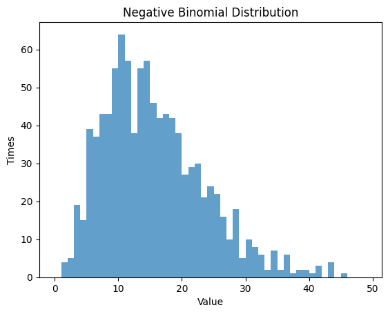
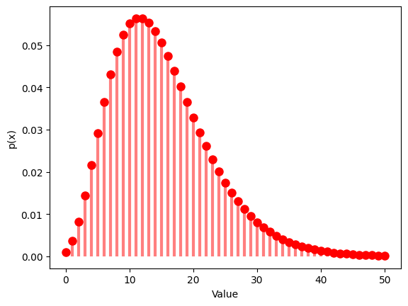
1.4.2 $p$ $=0.25$ , $n$ $=5$
1
2
3
4
5
6
7
8
9
10
11
12
13
14
15
16
17
18
19
20
| r = 5
p = 0.25
rv_nbinom = nbinom(r, p)
data_nbinom = rv_nbinom.rvs(size=1000)
# Randm Variable
plt.hist(data_nbinom, bins=np.arange(0, 50, 1), alpha=0.7)
plt.title('Negative Binomial Distribution')
plt.xlabel('Value')
plt.ylabel('Times')
plt.show()
# Probability mass function
x = np.arange(0, 51)
y = nbinom.pmf(x, r, p)
plt.plot(x, y, 'ro', ms=8)
plt.vlines(x, 0, y, colors='r', lw=3, alpha=0.5)
plt.xlabel('Value')
plt.ylabel('p(x)')
plt.show()
|
1
2
3
4
5
6
7
8
9
10
| theoretical_mean_nbinom = r * (1 - p) / p
theoretical_std_nbinom = np.sqrt(r * (1 - p) / (p ** 2))
mean_nbinom = np.mean(data_nbinom)
std_nbinom = np.std(data_nbinom)
print("\nNegative Binomial Distribution:")
print("Theoretical Mean:", theoretical_mean_nbinom)
print("Computed Mean:", mean_nbinom)
print("Theoretical Standard Deviation:", theoretical_std_nbinom)
print("Computed Standard Deviation:", std_nbinom)
|
1
2
3
4
5
| Negative Binomial Distribution:
Theoretical Mean: 15.0
Computed Mean: 15.204
Theoretical Standard Deviation: 7.745966692414834
Computed Standard Deviation: 7.9947722919417785
|
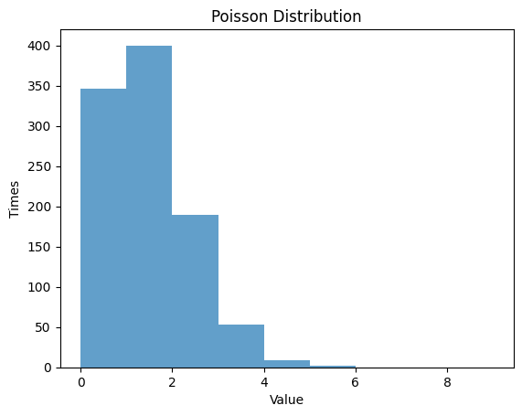
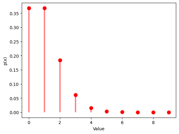
1.5 ポアソン分布
- ポアソン分布は、ある一定の時間や領域内で起こる事象の発生回数の確率分布です。
- 平均発生率 $λ$ を設定し、その分布を観察します。
1.5.1 $λ$ $=1$
1
2
3
4
5
6
7
8
9
10
11
12
13
14
15
16
17
18
19
| mu = 1 #lambda
rv_poisson = poisson(mu)
data_poisson = rv_poisson.rvs(size=1000)
# Randm Variable
plt.hist(data_poisson, bins=np.arange(0, 10, 1), alpha=0.7)
plt.title('Poisson Distribution')
plt.xlabel('Value')
plt.ylabel('Times')
plt.show()
# Probability mass function
x = np.arange(0, 10)
y = poisson.pmf(x, mu)
plt.plot(x, y, 'ro', ms=8)
plt.vlines(x, 0, y, colors='r', lw=3, alpha=0.5)
plt.xlabel('Value')
plt.ylabel('p(x)')
plt.show()
|
1
2
3
4
5
6
7
8
9
10
| theoretical_mean_poisson = mu
theoretical_std_poisson = np.sqrt(mu)
mean_poisson = np.mean(data_poisson)
std_poisson = np.std(data_poisson)
print("\nPoisson Distribution:")
print("Theoretical Mean:", theoretical_mean_poisson)
print("Computed Mean:", mean_poisson)
print("Theoretical Standard Deviation:", theoretical_std_poisson)
print("Computed Standard Deviation:", std_poisson)
|
1
2
3
4
5
| Poisson Distribution:
Theoretical Mean: 1
Computed Mean: 0.985
Theoretical Standard Deviation: 1.0
Computed Standard Deviation: 0.927779607449959
|
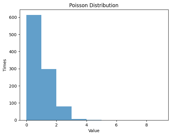
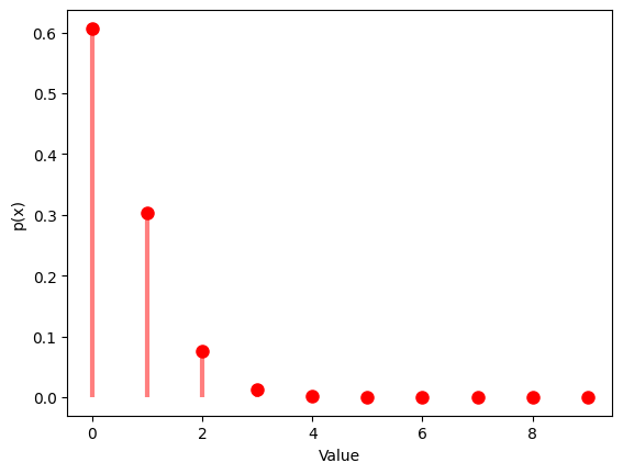
1.5.2 $λ$ $=0.5$
1
2
3
4
5
6
7
8
9
10
11
12
13
14
15
16
17
18
19
| mu = 0.5 #lambda
rv_poisson = poisson(mu)
data_poisson = rv_poisson.rvs(size=1000)
# Randm Variable
plt.hist(data_poisson, bins=np.arange(0, 10, 1), alpha=0.7)
plt.title('Poisson Distribution')
plt.xlabel('Value')
plt.ylabel('Times')
plt.show()
# Probability mass function
x = np.arange(0, 10)
y = poisson.pmf(x, mu)
plt.plot(x, y, 'ro', ms=8)
plt.vlines(x, 0, y, colors='r', lw=3, alpha=0.5)
plt.xlabel('Value')
plt.ylabel('p(x)')
plt.show()
|
1
2
3
4
5
6
7
8
9
10
| theoretical_mean_poisson = mu
theoretical_std_poisson = np.sqrt(mu)
mean_poisson = np.mean(data_poisson)
std_poisson = np.std(data_poisson)
print("\nPoisson Distribution:")
print("Theoretical Mean:", theoretical_mean_poisson)
print("Computed Mean:", mean_poisson)
print("Theoretical Standard Deviation:", theoretical_std_poisson)
print("Computed Standard Deviation:", std_poisson)
|
1
2
3
4
5
| Poisson Distribution:
Theoretical Mean: 0.5
Computed Mean: 0.483
Theoretical Standard Deviation: 0.7071067811865476
Computed Standard Deviation: 0.6809632882909327
|
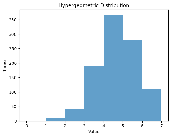
1.6 超幾何分布
- 超幾何分布は、有限個の要素の中から非復元抽出した場合、成功の数が従う確率分布です。
- 要素数 $N$,成功の数 $M$,抽出の数 $K$ を設計し、その分布を観察します。
1.6.1 $N$ $=20$ , $M$ $=7$ , $K$ $=12$
1
2
3
4
5
6
7
8
9
10
11
12
13
14
15
16
17
18
19
20
21
22
| N = 20 # the number of elements
M = 7 # the number of successes
K = 12 # the number of sample
rv_hypergeom = hypergeom(N, M, K)
data_hypergeom = rv_hypergeom.rvs(size=1000)
# Randm Variable
plt.hist(data_hypergeom, bins=np.arange(0, M+1, 1), alpha=0.7)
plt.title('Hypergeometric Distribution')
plt.xlabel('Value')
plt.ylabel('Times')
plt.show()
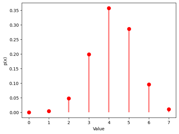
# Probability mass function
x = np.arange(max(0, K - (N - M)), min(M, K) + 1)
y = hypergeom.pmf(x, N, M, K)
plt.plot(x, y, 'ro', ms=8)
plt.vlines(x, 0, y, colors='r', lw=3, alpha=0.5)
plt.xlabel('Value')
plt.ylabel('p(x)')
plt.show()
|
1
2
3
4
5
6
7
8
9
10
| theoretical_mean_hypergeom = (M * K) / N;
theoretical_std_hypergeom = np.sqrt(((M * (N-M) * (N - K)) * (N - K)) / ((N - 1) * N**2))
mean_hypergeom = np.mean(data_hypergeom)
std_hypergeom = np.std(data_hypergeom)
print("\nHypergeom Distribution:")
print("Theoretical Mean:", theoretical_mean_hypergeom)
print("Computed Mean:", mean_hypergeom)
print("Theoretical Standard Deviation:", theoretical_std_hypergeom)
print("Computed Standard Deviation:", std_hypergeom)
|
1
2
3
4
5
| Hypergeom Distribution:
Theoretical Mean: 4.2
Computed Mean: 4.21
Theoretical Standard Deviation: 0.8753946478438649
Computed Standard Deviation: 1.0953994705129266
|
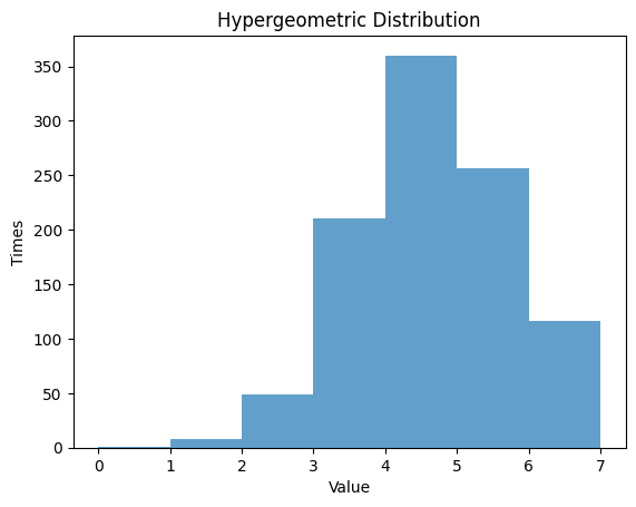
1.6.1 $N$ $=20$ , $M$ $=5$ , $K$ $=5$
1
2
3
4
5
6
7
8
9
10
11
12
13
14
15
16
17
18
19
20
21
22
| N = 20 # the number of elements
M = 7 # the number of successes
K = 12 # the number of sample
rv_hypergeom = hypergeom(N, M, K)
data_hypergeom = rv_hypergeom.rvs(size=1000)
# Randm Variable
plt.hist(data_hypergeom, bins=np.arange(0, M+1, 1), alpha=0.7)
plt.title('Hypergeometric Distribution')
plt.xlabel('Value')
plt.ylabel('Times')
plt.show()
# Probability mass function
x = np.arange(max(0, K - (N - M)), min(M, K) + 1)
y = hypergeom.pmf(x, N, M, K)
plt.plot(x, y, 'ro', ms=8)
plt.vlines(x, 0, y, colors='r', lw=3, alpha=0.5)
plt.xlabel('Value')
plt.ylabel('p(x)')
plt.show()
|
1
2
3
4
5
6
7
8
9
10
| theoretical_mean_hypergeom = (M * K) / N
theoretical_std_hypergeom = np.sqrt(((M * (N-M) * (N - K)) * (N - K)) / ((N - 1) * N**2))
mean_hypergeom = np.mean(data_hypergeom)
std_hypergeom = np.std(data_hypergeom)
print("\nHypergeom Distribution:")
print("Theoretical Mean:", theoretical_mean_hypergeom)
print("Computed Mean:", mean_hypergeom)
print("Theoretical Standard Deviation:", theoretical_std_hypergeom)
print("Computed Standard Deviation:", std_hypergeom)
|
1
2
3
4
5
| Hypergeom Distribution:
Theoretical Mean: 4.2
Computed Mean: 4.165
Theoretical Standard Deviation: 0.8753946478438649
Computed Standard Deviation: 1.1188275112813413
|
2.連続確率分布
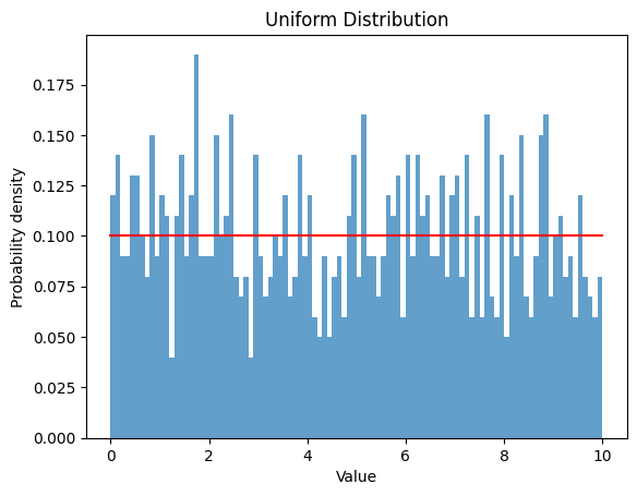
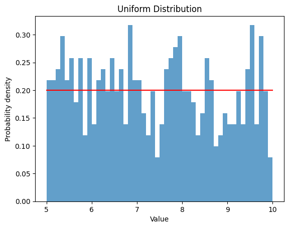
2.1 一様分布
- 一様分布は、範囲内の値がすべて同じ確率で起こる確率分布です。
- 下限 $a$ と上限 $b$ を設定し、その分布を観察します。
2.1.1 $a$ $=0$ , $b$ $=10$
1
2
3
4
5
6
7
8
9
10
11
12
13
14
| a = 0
b = 10
rv_uniform = uniform(a, b)
data_uniform = rv_uniform.rvs(size=1000)
plt.hist(data_uniform, bins=np.arange(a, b+0.1, 0.1), density=True, alpha=0.7)
x = np.linspace(a, b, 1000)
y = uniform.pdf(x, a, b-a)
plt.plot(x, y, color='red')
plt.title('Uniform Distribution')
plt.xlabel('Value')
plt.ylabel('Probability density')
plt.show()
|
1
2
3
4
5
6
7
8
9
10
11
| theoretical_mean_uniform = (a + b) / 2
theoretical_std_uniform = np.sqrt((b - a) ** 2 / 12)
mean_uniform = np.mean(data_uniform)
std_uniform = np.std(data_uniform)
print("\nUniform Distribution:")
print("Theoretical Mean:", theoretical_mean_uniform)
print("Computed Mean:", mean_uniform)
print("Theoretical Standard Deviation:", theoretical_std_uniform)
print("Computed Standard Deviation:", std_uniform)
|
1
2
3
4
5
| Uniform Distribution:
Theoretical Mean: 5.0
Computed Mean: 4.880078826205267
Theoretical Standard Deviation: 2.886751345948129
Computed Standard Deviation: 2.89996540104743
|
2.1.2 $a$ $=5$ , $b$ $=10$
1
2
3
4
5
6
7
8
9
10
11
12
13
14
| a = 5
b = 10
rv_uniform = uniform(a, b)
data_uniform = rv_uniform.rvs(size=1000)
plt.hist(data_uniform, bins=np.arange(a, b+0.1, 0.1), density=True, alpha=0.7)
x = np.linspace(a, b, 1000)
y = uniform.pdf(x, a, b-a)
plt.plot(x, y, color='red')
plt.title('Uniform Distribution')
plt.xlabel('Value')
plt.ylabel('Probability density')
plt.show()
|
1
2
3
4
5
6
7
8
9
10
11
| theoretical_mean_uniform = (a + b) / 2
theoretical_std_uniform = np.sqrt((b - a) ** 2 / 12)
mean_uniform = np.mean(data_uniform)
std_uniform = np.std(data_uniform)
print("\nUniform Distribution:")
print("Theoretical Mean:", theoretical_mean_uniform)
print("Computed Mean:", mean_uniform)
print("Theoretical Standard Deviation:", theoretical_std_uniform)
print("Computed Standard Deviation:", std_uniform)
|
1
2
3
4
5
| Uniform Distribution:
Theoretical Mean: 7.5
Computed Mean: 9.917425782206815
Theoretical Standard Deviation: 1.4433756729740645
Computed Standard Deviation: 2.9300814094272654
|
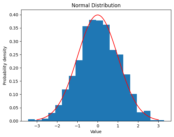
2.2 正規分布
- 釣り鐘型の分布です。\(f(x)=\frac{1}{\sqrt{2\pi\sigma}^2}e^{-\frac{(x-m)^2}{2\sigma^2}}\)
- 平均値 $m$ と標準偏差 $\sigma$ を設定し、その分布を観察します。
2.2.1 $m$ $=0 ,$ $\sigma$ $=1$
1
2
3
4
5
6
7
8
9
10
11
12
13
| mean = 0
std = 1
data_norm = norm.rvs(loc=mean, scale=std, size=1000)
plt.hist(data_norm, bins=20, density=True)
x = np.linspace(mean - 3*std, mean + 3*std, 100)
y = norm.pdf(x, loc=mean, scale=std)
plt.plot(x, y, color='red')
plt.xlabel('Value')
plt.ylabel('Probability density')
plt.title('Normal Distribution')
plt.show()
|
1
2
3
4
5
6
7
8
9
10
| theoretical_mean_norm = mean
theoretical_std_norm = std
mean_norm = np.mean(data_norm)
std_norm = np.std(data_norm)
print("\nNorm Distribution:")
print("Theoretical Mean:", theoretical_mean_norm)
print("Computed Mean:", mean_norm)
print("Theoretical Standard Deviation:", theoretical_std_norm)
print("Computed Standard Deviation:", std_norm)
|
1
2
3
4
5
| Norm Distribution:
Theoretical Mean: 0
Computed Mean: 0.0411486155486315
Theoretical Standard Deviation: 1
Computed Standard Deviation: 1.014172542912695
|
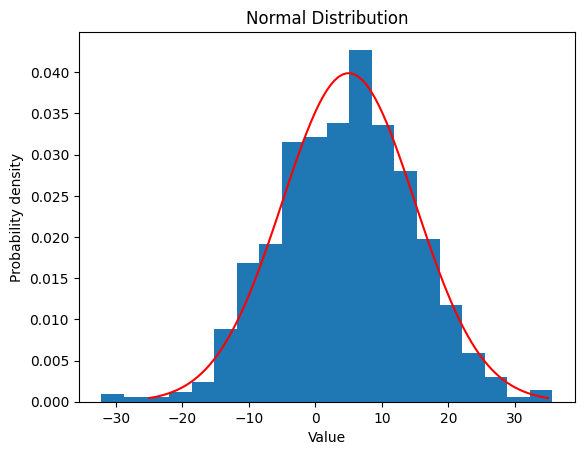
2.2.2 $m$ $=5 ,$ $\sigma$ $=10$
1
2
3
4
5
6
7
8
9
10
11
12
13
| mean = 5
std = 10
data = norm.rvs(loc=mean, scale=std, size=1000)
plt.hist(data, bins=20, density=True)
x = np.linspace(mean - 3*std, mean + 3*std, 100)
y = norm.pdf(x, loc=mean, scale=std)
plt.plot(x, y, color='red')
plt.xlabel('Value')
plt.ylabel('Probability density')
plt.title('Normal Distribution')
plt.show()
|
1
2
3
4
5
6
7
8
9
10
| theoretical_mean_norm = mean
theoretical_std_norm = std
mean_norm = np.mean(data_norm)
std_norm = np.std(data_norm)
print("\nNorm Distribution:")
print("Theoretical Mean:", theoretical_mean_norm)
print("Computed Mean:", mean_norm)
print("Theoretical Standard Deviation:", theoretical_std_norm)
print("Computed Standard Deviation:", std_norm)
|
1
2
3
4
5
| Norm Distribution:
Theoretical Mean: 5
Computed Mean: 0.0411486155486315
Theoretical Standard Deviation: 10
Computed Standard Deviation: 1.014172542912695
|
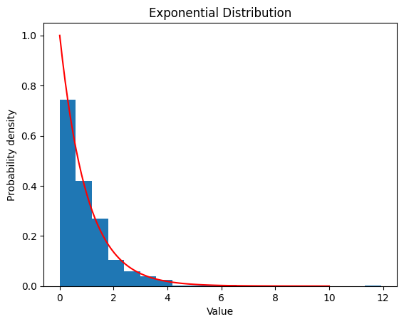
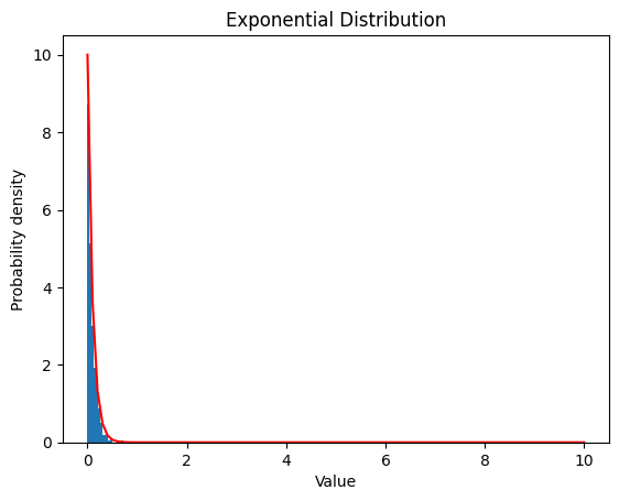
2.3 指数分布
\(f(x)=\begin{cases}λe^{-λ x},(x\ge 0)\\0 ,(x<0)\end{cases}\)
2.3.1 $λ$ $=1$
1
2
3
4
5
6
7
8
9
10
11
12
13
14
15
16
17
18
19
20
21
22
23
| lambda_ = 1
data_expon = expon.rvs(scale=1/lambda_, size=1000)
plt.hist(data_expon, bins=20, density=True)
x = np.linspace(0, 10, 100)
y = expon.pdf(x, scale=1/lambda_)
plt.plot(x, y, color='red')
plt.xlabel('Value')
plt.ylabel('Probability density')
plt.title('Exponential Distribution')
plt.show()
theoretical_mean_expon = 1 / lambda_
theoretical_std_expon = 1 / lambda_
mean_expon = np.mean(data_expon)
std_expon = np.std(data_expon)
print("\nExponential Distribution:")
print("Theoretical Mean:", theoretical_mean_expon)
print("Computed Mean:", mean_expon)
print("Theoretical Standard Deviation:", theoretical_std_expon)
print("Computed Standard Deviation:", std_expon)
|
1
2
3
4
5
| Exponential Distribution:
Theoretical Mean: 1.0
Computed Mean: 0.9885430257877893
Theoretical Standard Deviation: 1.0
Computed Standard Deviation: 1.018140760378851
|
2.3.2 $λ$ $=10$
1
2
3
4
5
6
7
8
9
10
11
12
13
14
15
16
17
18
19
20
21
22
| lambda_ = 10
data_expon = expon.rvs(scale=1/lambda_, size=1000)
plt.hist(data_expon, bins=20, density=True)
x = np.linspace(0, 10, 100)
y = expon.pdf(x, scale=1/lambda_)
plt.plot(x, y, color='red')
plt.xlabel('Value')
plt.ylabel('Probability density')
plt.title('Exponential Distribution')
plt.show()
theoretical_mean_expon = 1 / lambda_
theoretical_std_expon = 1 / lambda_
mean_expon = np.mean(data_expon)
std_expon = np.std(data_expon)
print("\nExponential Distribution:")
print("Theoretical Mean:", theoretical_mean_expon)
print("Computed Mean:", mean_expon)
print("Theoretical Standard Deviation:", theoretical_std_expon)
print("Computed Standard Deviation:", std_expon)
|
1
2
3
4
5
| Exponential Distribution:
Theoretical Mean: 0.1
Computed Mean: 0.09427400139219543
Theoretical Standard Deviation: 0.1
Computed Standard Deviation: 0.09509861055930452
|
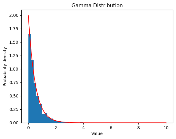
2.4 ガンマ分布
\(f(x)=\frac{1}{\Gamma(α)β^α}x^{α−1}e^{−x/β}\quad (x\ge0)\) $\Gamma(α)=∫_{0}^{∞}u^{α-1}e^{-u}du$
2.4.1 $α$ $=1 ,$ $β$ $=2$
1
2
3
4
5
6
7
8
9
10
11
12
13
14
15
16
17
18
19
20
21
22
23
| alpha = 1
beta = 2
data_gamma = gamma.rvs(a=alpha, scale=1/beta, size=1000)
plt.hist(data_gamma, bins=20, density=True)
x = np.linspace(0, 10, 100)
y = gamma.pdf(x, a=alpha, scale=1/beta)
plt.plot(x, y, color='red')
plt.xlabel('Value')
plt.ylabel('Probability density')
plt.title('Gamma Distribution')
plt.show()
theoretical_mean_gamma = alpha * beta
theoretical_std_gamma = np.sqrt(alpha) * beta
mean_gamma = np.mean(data_gamma)
std_gamma = np.std(data_gamma)
print("\nGamma Distribution:")
print("Theoretical Mean:", theoretical_mean_gamma)
print("Computed Mean:", mean_gamma)
print("Theoretical Standard Deviation:", theoretical_std_gamma)
print("Computed Standard Deviation:", std_gamma)
|
1
2
3
4
5
| Gamma Distribution:
Theoretical Mean: 2
Computed Mean: 0.5019967282218284
Theoretical Standard Deviation: 2.0
Computed Standard Deviation: 0.5109253271223613
|
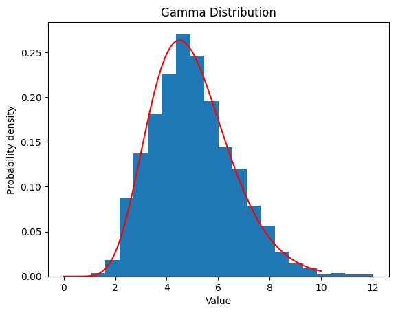
2.4.2 $α$ $=10 ,$ $β$ $=2$
1
2
3
4
5
6
7
8
9
10
11
12
13
14
15
16
17
18
19
20
21
22
23
| alpha = 10
beta = 2
data_gamma = gamma.rvs(a=alpha, scale=1/beta, size=1000)
plt.hist(data_gamma, bins=20, density=True)
x = np.linspace(0, 10, 100)
y = gamma.pdf(x, a=alpha, scale=1/beta)
plt.plot(x, y, color='red')
plt.xlabel('Value')
plt.ylabel('Probability density')
plt.title('Gamma Distribution')
plt.show()
theoretical_mean_gamma = alpha * beta
theoretical_std_gamma = np.sqrt(alpha) * beta
mean_gamma = np.mean(data_gamma)
std_gamma = np.std(data_gamma)
print("\nGamma Distribution:")
print("Theoretical Mean:", theoretical_mean_gamma)
print("Computed Mean:", mean_gamma)
print("Theoretical Standard Deviation:", theoretical_std_gamma)
print("Computed Standard Deviation:", std_gamma)
|
1
2
3
4
5
| Gamma Distribution:
Theoretical Mean: 20
Computed Mean: 5.031567622623559
Theoretical Standard Deviation: 6.324555320336759
Computed Standard Deviation: 1.6000337136252216
|
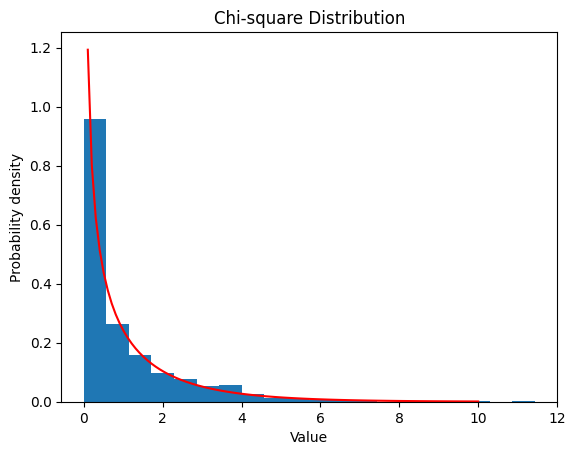
2.5 カイ二乗分布
\(f(x)=\frac{1}{2^{ν/2}Γ(ν/2)}x^{ν/2−1}e^{−x/2}\quad (x\ge 0)\)
2.5.1 $ν$ $=1$
1
2
3
4
5
6
7
8
9
10
11
12
13
14
15
16
17
18
19
20
21
22
| nu = 1
data_chisq = chi2.rvs(df=nu, size=1000)
plt.hist(data_chisq, bins=20, density=True)
x = np.linspace(0, 10, 100)
y = chi2.pdf(x, df=nu)
plt.plot(x, y, color='red')
plt.xlabel('Value')
plt.ylabel('Probability density')
plt.title('Chi-square Distribution')
plt.show()
theoretical_mean_chisq = nu
theoretical_std_chisq = np.sqrt(2 * nu)
mean_chisq = np.mean(data_chisq)
std_chisq = np.std(data_chisq)
print("\nChi-square Distribution:")
print("Theoretical Mean:", theoretical_mean_chisq)
print("Computed Mean:", mean_chisq)
print("Theoretical Standard Deviation:", theoretical_std_chisq)
print("Computed Standard Deviation:", std_chisq)
|
1
2
3
4
5
| Chi-square Distribution:
Theoretical Mean: 1
Computed Mean: 1.0659771170216892
Theoretical Standard Deviation: 1.4142135623730951
Computed Standard Deviation: 1.4809657924560946
|
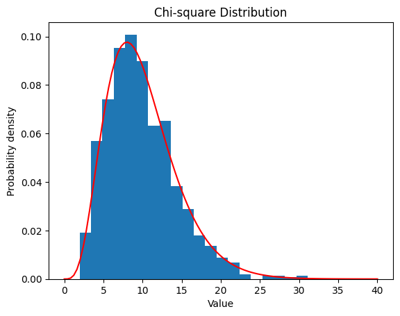
2.5.2 $ν$ $=10$
1
2
3
4
5
6
7
8
9
10
11
12
13
14
15
16
17
18
19
20
21
22
| nu = 10
data_chisq = chi2.rvs(df=nu, size=1000)
plt.hist(data_chisq, bins=20, density=True)
x = np.linspace(0, 40, 100)
y = chi2.pdf(x, df=nu)
plt.plot(x, y, color='red')
plt.xlabel('Value')
plt.ylabel('Probability density')
plt.title('Chi-square Distribution')
plt.show()
theoretical_mean_chisq = nu
theoretical_std_chisq = np.sqrt(2 * nu)
mean_chisq = np.mean(data_chisq)
std_chisq = np.std(data_chisq)
print("\nChi-square Distribution:")
print("Theoretical Mean:", theoretical_mean_chisq)
print("Computed Mean:", mean_chisq)
print("Theoretical Standard Deviation:", theoretical_std_chisq)
print("Computed Standard Deviation:", std_chisq)
|
1
2
3
4
5
| Chi-square Distribution:
Theoretical Mean: 10
Computed Mean: 9.857850290941526
Theoretical Standard Deviation: 4.47213595499958
Computed Standard Deviation: 4.455651979640904
|