Optimal Control Problem
Unicycle Model
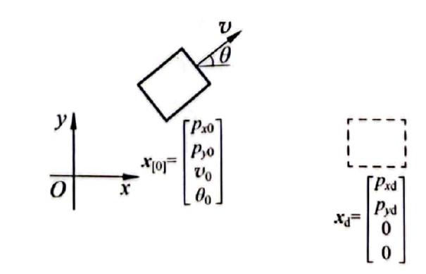
State Space
\[x(t)=\begin{bmatrix} x_1(t)\\ x_2(t)\\ x_3(t)\\ x_4(t) \end{bmatrix}=\begin{bmatrix} p_x(t)\\ p_y(t)\\ v(t)\\ \theta(t) \end{bmatrix}\]- $p_x(t)$: position in x direction
- $p_y(t)$: position on y direction
- $v(t)$: linear velocity
- $\theta(t)$: the wheel orientation
Input
\[u(t)=\begin{bmatrix} u_1(t)\\ u_2(t)\\ \end{bmatrix}=\begin{bmatrix} \alpha(t)\\ \omega(t)\\ \end{bmatrix}\]- $\alpha(t)$: acceleration
- $\omega(t)$: angular velocity
State space
\[\dot x(t)=\begin{bmatrix} v(t)\cos{\theta(t)}\\ v(t)\sin{\theta(t)}\\ 0\\0 \end{bmatrix}+\begin{bmatrix} 0\\ 0\\ \alpha(t)\\\omega(t) \end{bmatrix}=f(x(t),u(t))\]nonlinear System
Discretization
- $T_s$: sample time
- $f_d$ is discrete-time
Problem 1: Parking problem
- System
- $x[0]:$ Initial states
- $x_d:$ Reference value
$k\to N$: Terminal state $x[N]$
\[x[N]=f_d[\dots[f_d[x[0],u[0],u[1],\dots,u[N-1]]]]\]The final states are only related to the initial states and inputs
Performance function
\[\begin{aligned}J&=(x_1[N]-x_{d1})^2+(x_2[N]-x_{d2})^2+(x_3[N]-x_{d3})^2+(x_4[N]-x_{d4})^2\\&=(x[N]-x_d)^T(x[N]-x_d)=\|x[N]-x_d\|^2\\&=e[N]^Te[N]=\|e[N]\|^2\end{aligned}\]- $e[k]$: error \(e[k]=x[k]-x_d\)
$J$ is also called cost function.
Control Policy
Optimal input:
- $u^*\in\Omega$: input in the set of Admissible Control
Weight matrix
By using the weight matrix, we can decide which states are more important. We obtain a new performance function as:
\[J=e[N]^TSe[N]\triangleq\|x[N]-x_d\|^2_S\]- $S$: weight matrix
- Positive Semi-Definite symmetric matrix $x^TSx\ge0\;and\;s_{ij}=s_{ji}$
In fact, $S$ is usually a diagonal matrix. $for\;i\ne j \to s_{ij}=0$
Constraints
physical constraints
\[-v_{max}<v[k]<v_{max}\] \[u_{min}<u[k]<u_{max}\]Hard constraints: The constraint condition must be strictly satisfied in the system control.
Problem 2: Consider the cost of input under Problem 1
Soft Constraints: The constraint condition isn’t strictly satisfied in the system control.
\[J=\|x[N]-x_d\|^2_S+\sum_{k=0}^{N-1}\|u[k]\|^2_R\]- $|x[N]-x_d|^2_S=(x[N]-x_d)^TS(x[N]-x_d)$
$|u[k]|^2_R=u[k]^TRu[k]$
- $S:$ reference weight matrix
- $R:$ cost weight matrix
$S>R:$ The control performance is more important!
$R>S:$ The cost of input is more important!
Problem 3:Trajectory under Scenario 1 and 2
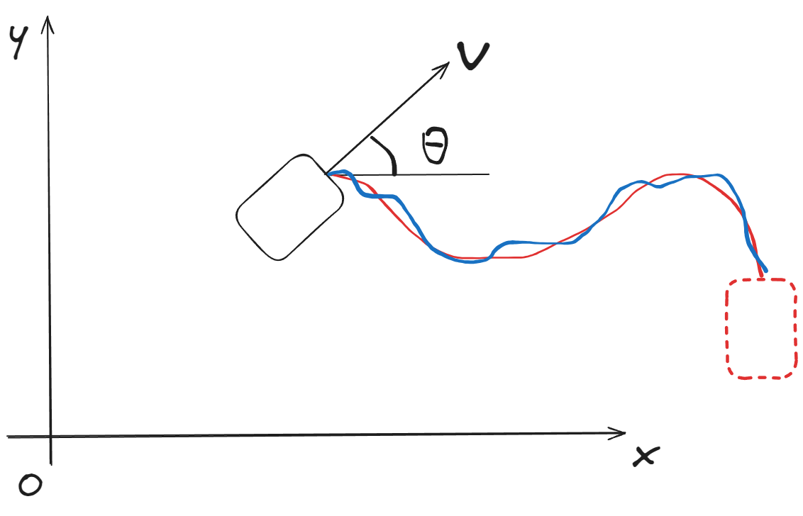
Reference trajectory:
\[x_d[k]=\begin{bmatrix}p_{xd}[k]\\p_{yd}[k]\\0\\0\end{bmatrix}\]Performance function \(J=\|x[N]-x_d\|^2_S+\sum_k^{N-1}\left(\|x[k]-x_d[k]\|_Q^2+\|u[k]\|^2_R\right)\)
$Q$: Trajectory weight matrix
Problem 4:Collision Avoidance
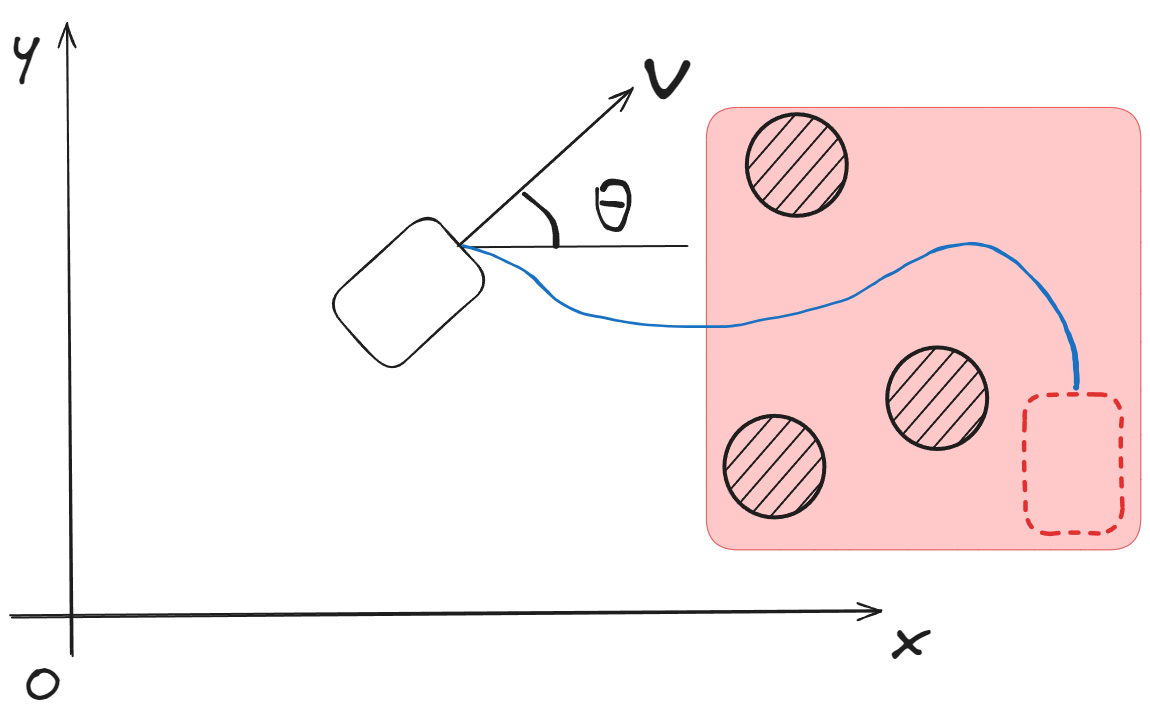
Method 1: Add constraint condition
Add constraint condition for the performance function in Problem 3
\[(p_x[k],p_y[k])\notin (p_{xo},p_{yo})\]- $(p_{xo},p_{yo})\in\Omega_o:$ Obstacle space
Method 2: Add soft constraints
Add soft constraints to limit the distance from the control object to the obstacle.
\[J=\|x[N]-x_d\|^2_S+\sum_k^{N-1}\left(\|x[k]-x_d[k]\|_Q^2+\|u[k]\|^2_R\right)+D^{-1}[k]_{P}\]- $D[k]$: The distance from the object to the obstacle during movement
- $P:$ weight matrix for $D^{-1}$
Summary for optimal control problem
- System model: state space expression
- Reference $x_d[k]$
- Performance function (cost function)
- Constaints condition
- $x[k]\in X$, where $X$ is admissible trajectory
- $u[k]\in \Omega$, where $\Omega$ is set of admissible control
Notes that there is at least a feasible solution within the constraints. Otherwise, too strict constraints will lead to no solution for problem.
Common optimal control problems
The shortest time problem
\[J=\sum^N1=N\]Terminal control problem
\[J=\|x[N]-x_d[N]\|_S^2\]Minimum input problem
\[J=\sum_{k=0}^{N}\|u[k]\|_{R[k]}^2\]Trajectory problem
\[J=\sum_{k=0}^{N}\|x[k]-x_d[k]\|_{Q[k]}^2\]Multiple problem
\[J=\|x[N]-x_d[N]\|_S^2+\sum_{k=0}^{N-1}\left(\|x[k]-x_d[k]\|_{Q[k]}^2+\|u[k]\|_{R[k]}^2\right)\]Regulator problem
\[J=\|x[N]\|_S^2+\sum_{k=0}^{N-1}\left(\|x[k]-x_d[k]\|_{Q[k]}^2+\|u[k]\|_{R[k]}^2\right)\]When $x_d[k]=0$, it’s called regulator problem.
For trajectory problem, We can Introduce error $e[k]=x[k]-x_d[k]$ and state space for error. Then, control task becomes $e[k]\to0$. Therefor, the problem can solution as a regulator problem.
Reference
- Optimal Control by DR_CAN
- 王天威. 控制之美(卷 2). 清华大学出版社,2023.
- Grune L. Dynamic programming, optimal control and model predictive control. Springer, 2018.
- Kirk D. Optimal control theory: An introduction. Dover Publications, 2004