Model Predictive Control
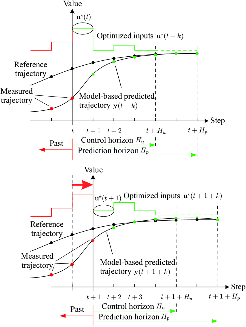
Model Predictive Control (MPC), known as Receding Horizon Control, is a method that involves solving an optimal control problem over a finite prediction horizon at each sampling time to calculate the optimal control sequence. Only the first control in this sequence is applied, and the process repeats at the next sampling time.
SISO Discrete-time System
State-space equation:
\[x_{[k+1]}=f(x_{[k]},u_{[k]})\]Performance function:
\[J=h(x_{[N]},x_d)+\sum_{k=1}^{N_p-1}g(x_{[k]},x_d,u_{[k]})\]- Prediction horizon: $N_p$
- Control horizon: $N_c$
Commonly, we set $N_p=N_c$.
At each time step $k$, the MPC algorithm performs two main tasks:
Control Calculation: It calculates the optimal control sequence ( $u_{[k \mid k]}$, $u_{[ k+1 \mid k]}$, $\dots$, $u_{[k+N_c-1 \mid k]}$ ), considering the current state $x_{[k]}$ and the prediction horizon. $N_c$ is the control horizon.
State Prediction: It utilizes the system model (state-space equation) and the calculated control sequence to predict the future system states ( $x_{[k+1\mid k]}$, $x_{[k+2\mid k]}$, $\dots$, $x_{[k+N_p\mid k]}$ ). $N_p$ is the prediction horizon.
It means for time step $k+1$. MPC calculates the optimal control sequence ( $u_{[k+1\mid k+1]}$, $u_{[k+2\mid k+1]}$, $\dots$, $u_{[k+N_c\mid k+1]}$ ) and predicts the system states ( $x_{[k+2\mid k+1]}$, $x_{[k+3\mid k+1]}$, $\dots$, $x_{[k+1+N_p\mid k+1]}$ ).
Notices that $u_{[k+i\mid k]}$ represents the control action calculated at time step $k$ to be applied at time step $k+i$. $x_{[k+i\mid k]}$ represents the state predicted at time step $k$ for time step $k+i$.
Quadratic Programming
MPC often relies on solving a QP problem at each time step to determine the optimal control actions.
A quadratic program(QP) is the problem of optimizing a quadratic objective function subject to linear constraints. Mathematically,
\[\text{Minimize}: J= \frac{1}{2}x^TQx+R^Tx\] \[\text{subject to}: Ax\le b,\; A_{eq}x=b_{eq},\; x_L \le x\le x_U\]where $x\in\mathbb{R}^n$ is the vector of design variables. The remaining matrices/vectors have dimensions $Q\in\mathbb{R}^n$ , $R\in\mathbb{R}^n$, $S\in\mathbb{R}$, $A\in \mathbb{R}^{m\times n}$, $b\in\mathbb{R}^m$, $A_{eq}\in \mathbb{R}^{l\times n}$, $b\in\mathbb{R}^l$, where $n$ is the number of design variables, $m$ is the number of inequality constraints, and $l$ is the number of equality constraints. $x_L,x_U$ are lower bound and upper bound of design variables.
A. Non Constraints
When there are no constraints and $Q$ is a positive definite matrix and has inverse matrix.
\[\frac{\partial J}{\partial x}=0\] \[\implies Qx+R=0\implies x^\ast=-Q^{-1}R\] \[\frac{\partial^2 J}{\partial^2 x}=Q>0\]B. Equality Constraints
Lagrange multiplier
When there are equality constraints $A_{eq}x= b_{eq}$, Lagrange multiplier - Wikipedia can solve it.
\[J=\frac{1}{2}x^TQx+R^Tx, \; A_{eq}x=b_{eq}\]The Lagrangian function is defined as
\[L=\frac{1}{2}x^TQx+R^Tx+\lambda^T(A_{eq}x-b_{eq})\]All partial derivatives should be zero:
\[\frac{\partial L}{\partial x}=Qx+R+A_{eq}^T\lambda=0\] \[\frac{\partial L}{\partial \lambda}=A_{eq}x-b_{eq}=0\]Then, we have the following equation.
\[\begin{bmatrix} Q & A_{eq}^T\\ A_{eq} & 0 \end{bmatrix}\begin{bmatrix} x\\\lambda \end{bmatrix}=\begin{bmatrix} -R\\ b_{eq} \end{bmatrix}\]If there is the inverse matrix, we can calculate the results as
\[\begin{bmatrix} x^\ast\\ \lambda^\ast \end{bmatrix}=\begin{bmatrix} Q & A_{eq}^T\\ A_{eq} & 0 \end{bmatrix}^{-1}\begin{bmatrix} -R\\ b_{eq} \end{bmatrix}\]C. Inequality Constraints
For optimization problems with inequality constraints, obtaining an analytical solution is often difficult. In such cases, a numerical solution can be used. Common numerical methods include the interior-point method, gradient method, and Newton method. These methods are easy to implement in software such as MATLAB, Octave, and Python.
MATLAB
quadprog - Quadratic programming - MATLAB (mathworks.com)
1
x = quadprog(Q,R,A,b,Aeq,beq,xL,xU)
CasADi
An open-source tool for nonlinear optimization and algorithmic differentiation. (Support MATLAB/Octave, Python)
Reference
- Rakovic, S. V., & Levine, W. S. Handbook of model predictive control. 2018.
- CH02-QuadraticProgramming.pdf (berkeley.edu)

