問題と背景
Titanic - Machine Learning from Disaster
問題:機械学習により、タイタニック号の遭難事故で生き残った乗客を予測するモデルを作成する.
背景:Kaggle試合「Titanic - Machine Learning from Disaster」のDescriptionには,「On April 15, 1912, during her maiden voyage, the widely considered “unsinkable” RMS Titanic sank after colliding with an iceberg. Unfortunately, there weren’t enough lifeboats for everyone onboard, resulting in the death of 1502 out of 2224 passengers and crew.」と述べられている.
運の要素もあるが,女性,子供,上流階級などは,他のグループと比べて生き延びる可能性が高いことが一般的に考えられる.
機械学習最終レポート 氏名:YANG GUANGZE 学籍番号:20T1126N
More about machine-lerning | Github
分析開始
1
2
3
4
5
6
7
8
9
10
| # ライブラリーのインポート
import numpy as np
import pandas as pd
import matplotlib.pyplot as plt
import seaborn as sns
%matplotlib inline
#赤いwarmを消すため
import warnings
warnings.filterwarnings("ignore")
|
1
2
3
| # JupyterNotebookの表示領域
pd.set_option("display.max_columns", 100)
pd.set_option("display.max_rows", 100)
|
1
2
3
4
| # データの読込み
train_df = pd.read_csv("./train.csv")
test_df = pd.read_csv("./test.csv")
train_df.head(10) # 先頭部分の表示
|
| PassengerId | Survived | Pclass | Name | Sex | Age | SibSp | Parch | Ticket | Fare | Cabin | Embarked |
|---|
| 0 | 1 | 0 | 3 | Braund, Mr. Owen Harris | male | 22.0 | 1 | 0 | A/5 21171 | 7.2500 | NaN | S |
|---|
| 1 | 2 | 1 | 1 | Cumings, Mrs. John Bradley (Florence Briggs Th... | female | 38.0 | 1 | 0 | PC 17599 | 71.2833 | C85 | C |
|---|
| 2 | 3 | 1 | 3 | Heikkinen, Miss. Laina | female | 26.0 | 0 | 0 | STON/O2. 3101282 | 7.9250 | NaN | S |
|---|
| 3 | 4 | 1 | 1 | Futrelle, Mrs. Jacques Heath (Lily May Peel) | female | 35.0 | 1 | 0 | 113803 | 53.1000 | C123 | S |
|---|
| 4 | 5 | 0 | 3 | Allen, Mr. William Henry | male | 35.0 | 0 | 0 | 373450 | 8.0500 | NaN | S |
|---|
| 5 | 6 | 0 | 3 | Moran, Mr. James | male | NaN | 0 | 0 | 330877 | 8.4583 | NaN | Q |
|---|
| 6 | 7 | 0 | 1 | McCarthy, Mr. Timothy J | male | 54.0 | 0 | 0 | 17463 | 51.8625 | E46 | S |
|---|
| 7 | 8 | 0 | 3 | Palsson, Master. Gosta Leonard | male | 2.0 | 3 | 1 | 349909 | 21.0750 | NaN | S |
|---|
| 8 | 9 | 1 | 3 | Johnson, Mrs. Oscar W (Elisabeth Vilhelmina Berg) | female | 27.0 | 0 | 2 | 347742 | 11.1333 | NaN | S |
|---|
| 9 | 10 | 1 | 2 | Nasser, Mrs. Nicholas (Adele Achem) | female | 14.0 | 1 | 0 | 237736 | 30.0708 | NaN | C |
|---|
1
2
3
| # データのサイズ
print(train_df.shape)
print(test_df.shape)
|
分析説明:
データにより,一つの目標変数「Survived」に対して,説明変数「PassengerId」,「Pclass」,「Name」,「Sex」,「Age」,「SibSp」,「Parch」,「Ticket」,「Fare」,「Cabin」,「Embarked」がある.
日本語にすると,搭乗者番号,搭乗者階級,搭乗者氏名,性別,年齢,同乗した兄弟と配偶者の数,同乗した両親と子供の数,チケット番号,運賃,客室番号,乗車した港である.
よって,今回では,上記の説明変数を用いて目標変数「Survived」を予測する機械学習の判別問題をする.
また,学習データ891個,テストデータ418個である
内容については,以下のようになる.
1.学習データへの理解
2.説明変数の加工
3.機械学習
4.Kaggle最終結果
1.学習データへの理解
1.1データを確認する
説明変数のデータ型とデータの欠損について考察することで,加工すべきな説明変数を探す.
1
2
| train_df.dtypes # データの型を表示
train_df.info() # データの詳細を表示
|
1
2
3
4
5
6
7
8
9
10
11
12
13
14
15
16
17
18
19
| <class 'pandas.core.frame.DataFrame'>
RangeIndex: 891 entries, 0 to 890
Data columns (total 12 columns):
# Column Non-Null Count Dtype
--- ------ -------------- -----
0 PassengerId 891 non-null int64
1 Survived 891 non-null int64
2 Pclass 891 non-null int64
3 Name 891 non-null object
4 Sex 891 non-null object
5 Age 714 non-null float64
6 SibSp 891 non-null int64
7 Parch 891 non-null int64
8 Ticket 891 non-null object
9 Fare 891 non-null float64
10 Cabin 204 non-null object
11 Embarked 889 non-null object
dtypes: float64(2), int64(5), object(5)
memory usage: 83.7+ KB
|
1
2
| test_df.dtypes # データの型を表示
test_df.info() # データの詳細を表示
|
1
2
3
4
5
6
7
8
9
10
11
12
13
14
15
16
17
18
| <class 'pandas.core.frame.DataFrame'>
RangeIndex: 418 entries, 0 to 417
Data columns (total 11 columns):
# Column Non-Null Count Dtype
--- ------ -------------- -----
0 PassengerId 418 non-null int64
1 Pclass 418 non-null int64
2 Name 418 non-null object
3 Sex 418 non-null object
4 Age 332 non-null float64
5 SibSp 418 non-null int64
6 Parch 418 non-null int64
7 Ticket 418 non-null object
8 Fare 417 non-null float64
9 Cabin 91 non-null object
10 Embarked 418 non-null object
dtypes: float64(2), int64(4), object(5)
memory usage: 36.0+ KB
|
よって,以下の3点をまとめられる.
1.データの型について「Name」,「Sex」,「Ticket」,「Cabin」,「Embarked」はobject型なので,説明変数の加工(ダミー変数への変換)が必要である.
2.データの損失について「Age」,「Fare」はデータの欠損があるので,説明変数の加工(欠損値 の置き換え)が必要である.
3.「Cabin」の欠損が大きいので,「Cabin」を重要な要素として扱わない方が良いと考える.
1.2データの分布,目標変換との関係
データ変数の分布を考察することで,各変数を深く理解する.
1.2.1 目標変数「Survived」に対して
1
2
| # 学習データにおける生存率(1:生存, 0:故人)
train_df["Survived"].mean()
|
学習データの生存率は,約38%であることをわかった.
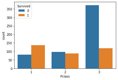
1.2.2 説明変数Pclassに対して
階級により,身分の高さが目標変数「Survived」に大きく影響を与えると期待する.
また,階級による経済的な差もあるので,チケット番号,運賃,客室番号に影響を及ぼすことを予想する. チケット番号,運賃,客室番号は,階級による間接効果であると仮説する.
1
2
| # 要素の頻度
train_df["Pclass"].value_counts()
|
1
2
3
4
| 3 491
1 216
2 184
Name: Pclass, dtype: int64
|
1
2
3
| # Pclass別の生存数カウント
import seaborn as sns
sns.countplot(data=train_df, x="Pclass", hue="Survived");
|
1
2
| # Pclass別の生存率
train_df["Survived"].groupby(train_df["Pclass"]).mean()
|
1
2
3
4
5
| Pclass
1 0.629630
2 0.472826
3 0.242363
Name: Survived, dtype: float64
|
結果:説明変数の「Pclass」別により,生存率が大幅に異なっていることをわかった.
よって,階級が高い(1>2>3)の方が生き延びる可能性が高いことが明らかになっている.Pclassは非常に重要な変数である.
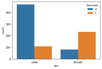
1.2.3 説明変数Sexに対して
性別により,目標変数「Survived」に大きく影響を与えると期待する.理由として,欧米の文化には「adies first」が存在しているためである.
1
2
| # Sex別の生存数カウント(1:生存, 0:故人)
sns.countplot(data=train_df, x="Sex", hue="Survived");
|
1
2
| # 要素の頻度
train_df["Sex"].value_counts()
|
1
2
3
| male 577
female 314
Name: Sex, dtype: int64
|
1
2
| # Sex別の生存率
train_df["Survived"].groupby(train_df["Sex"]).mean()
|
1
2
3
4
| Sex
female 0.742038
male 0.188908
Name: Survived, dtype: float64
|
結果:予想通りに,女性の方が生存率がとても高いことをわかった.
ただし,この影響は,性別の直接効果か階級による性別の間接効果かを考察すべきだと考える.
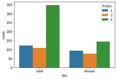
1
2
| # Sex別のPclassカウント
sns.countplot(data=train_df, x="Sex",hue="Pclass");
|
この図により,男性の中に階級が低いの方が多いのに,女性の方が生存率が高いということは,確かに性別の直接効果(female>male)である.階級より影響力が高い要素かもしれない.
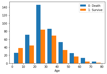
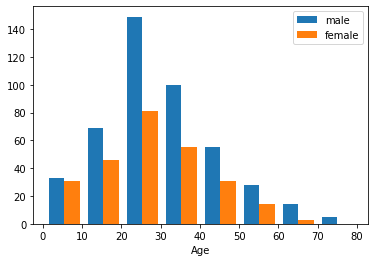
1.2.4 説明変数Ageに対して
年齢により,目標変数「Survived」に大きく影響を与えると期待する.理由として,「子供を優先すること」が存在しているためである.
1
2
3
| # Ageの抽出
Age0 = train_df[ train_df["Survived"]==0 ]["Age"]
Age1 = train_df[ train_df["Survived"]==1 ]["Age"]
|
1
2
3
4
| # ヒストグラム
plt.hist( [Age0, Age1], bins=8, label=["0: Death", "1: Survive"] )
plt.legend()
plt.xlabel("Age");
|
結果:予想通りに若いほど生き延びる可能性が高いことをわかった.
ただし,この影響は,年齢の直接効果か間接効果かを考察すべきだと考える.
1
2
3
| # AgeとSexの関係
Age2 = train_df[ train_df["Sex"]=="male" ]["Age"]
Age3 = train_df[ train_df["Sex"]=="female" ]["Age"]
|
1
2
3
4
| # ヒストグラム
plt.hist( [Age2, Age3], bins=8, label=["male", "female"] )
plt.legend()
plt.xlabel("Age");
|
1
2
3
4
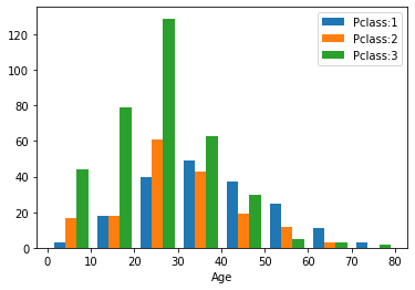
| # AgeとPclassの関係
Age4 = train_df[ train_df["Pclass"]==1 ]["Age"]
Age5 = train_df[ train_df["Pclass"]==2 ]["Age"]
Age6 = train_df[ train_df["Pclass"]==3 ]["Age"]
|
1
2
3
4
| # ヒストグラム
plt.hist( [Age4, Age5, Age6], bins=8, label=["Pclass:1", "Pclass:2","Pclass:3"] )
plt.legend()
plt.xlabel("Age");
|
これによって,年齢ごとに,階級と性別の偏りがないので,若いほど生き延びる可能性が高いことは,年齢の直接効果だと考えられる.
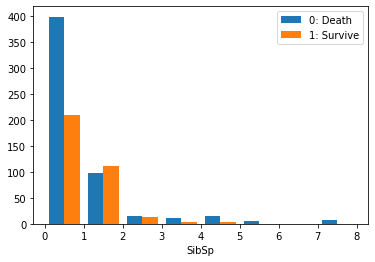
1.2.5 説明変数SibSp,Parchに対して
同乗した兄弟,配偶者,両親,子供の数は,生存率に大きく影響されないと考えられるが,これらのデータを考察する
1
2
| # SibSp別の生存率
train_df["Survived"].groupby(train_df["SibSp"]).mean()
|
1
2
3
4
5
6
7
8
9
| SibSp
0 0.345395
1 0.535885
2 0.464286
3 0.250000
4 0.166667
5 0.000000
8 0.000000
Name: Survived, dtype: float64
|
1
2
| # 要素の頻度
train_df["SibSp"].value_counts()
|
1
2
3
4
5
6
7
8
| 0 608
1 209
2 28
4 18
3 16
8 7
5 5
Name: SibSp, dtype: int64
|
1
2
3
4
5
6
7
| # SibSpの抽出
SibSp0 = train_df[ train_df["Survived"]==0 ]["SibSp"]
SibSp1 = train_df[ train_df["Survived"]==1 ]["SibSp"]
# ヒストグラム
plt.hist( [SibSp0, SibSp1], bins=8, label=["0: Death", "1: Survive"] )
plt.legend()
plt.xlabel("SibSp");
|
1
2
| # Parch別の生存率
train_df["Survived"].groupby(train_df["Parch"]).mean()
|
1
2
3
4
5
6
7
8
9
| Parch
0 0.343658
1 0.550847
2 0.500000
3 0.600000
4 0.000000
5 0.200000
6 0.000000
Name: Survived, dtype: float64
|
1
2
| # 要素の頻度
train_df["Parch"].value_counts()
|
1
2
3
4
5
6
7
8
| 0 678
1 118
2 80
5 5
3 5
4 4
6 1
Name: Parch, dtype: int64
|
1
2
3
4
5
6
7
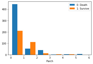
| # Parchの抽出
Parch0 = train_df[ train_df["Survived"]==0 ]["Parch"]
Parch1 = train_df[ train_df["Survived"]==1 ]["SibSp"]
# ヒストグラム
plt.hist( [Parch0, Parch1], bins=6, label=["0: Death", "1: Survive"] )
plt.legend()
plt.xlabel("Parch");
|
結果:要素の頻度により,同乗した兄弟,配偶者,両親,子供の数が多いの方が少ないので,参考にならない.さらに同乗した兄弟,配偶者,両親,子供の数と生存率の関係は,明らかに線形的ではない.しかしながら,家族の有無は,生存率に影響を与えると考えられる.
説明変数SibSp,Parchに対して,新しな説明変数「Family」で家族の有無を表示すれば,機械学習モデルの正確さを高めるだろう.
1.2.6 説明変数Fareに対して
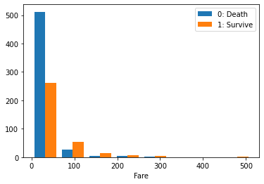
運賃が生存率に若干影響を与えると予想される.理由としては,運賃の高さも階級を表すと考えっている.
1
2
3
4
5
6
7
| # Fareの抽出
Fare0 = train_df[ train_df["Survived"]==0 ]["Fare"]
Fare1 = train_df[ train_df["Survived"]==1 ]["Fare"]
# ヒストグラム
plt.hist( [Fare0, Fare1], bins=8, label=["0: Death", "1: Survive"] )
plt.legend()
plt.xlabel("Fare");
|
結果:予想通りに,運賃が高い方が生き延びる可能性が高いかもしれない.
そして,この影響が運賃の直接効果か階級による間接効果かを考察する.
1
2
3
4
5
6
7
8
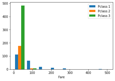
| # FareとPclassの関係
Fare2 = train_df[ train_df["Pclass"]==1 ]["Fare"]
Fare3 = train_df[ train_df["Pclass"]==2 ]["Fare"]
Fare4 = train_df[ train_df["Pclass"]==3 ]["Fare"]
# ヒストグラム
plt.hist( [Fare2, Fare3, Fare4], bins=8, label=["Pclass:1", "Pclass:2","Pclass:3"] )
plt.legend()
plt.xlabel("Fare");
|
これによって,運賃は階級ごとに明らかな偏りが存在しているので,運賃の影響は階級による間接効果だと考えられる
機械学習モデルの正確さを高めるために,Fare要素の重さを小さくする方が良いかもしれない.
1.2.7 説明変数Name,Ticket,Cabin,Embarkedに対して
名前,チケット番号,客室番号,乗車した港は,生存率にあまり影響を及ばないと予想される.理由は,これらのデータが多様な文字列としてルールがない.
1
2
| # データの確認
train_df["Name"].head()
|
1
2
3
4
5
6
| 0 Braund, Mr. Owen Harris
1 Cumings, Mrs. John Bradley (Florence Briggs Th...
2 Heikkinen, Miss. Laina
3 Futrelle, Mrs. Jacques Heath (Lily May Peel)
4 Allen, Mr. William Henry
Name: Name, dtype: object
|
1
2
| # 要素毎のデータ数
train_df["Name"].value_counts()
|
1
2
3
4
5
6
7
8
9
10
11
12
| Braund, Mr. Owen Harris 1
Boulos, Mr. Hanna 1
Frolicher-Stehli, Mr. Maxmillian 1
Gilinski, Mr. Eliezer 1
Murdlin, Mr. Joseph 1
..
Kelly, Miss. Anna Katherine "Annie Kate" 1
McCoy, Mr. Bernard 1
Johnson, Mr. William Cahoone Jr 1
Keane, Miss. Nora A 1
Dooley, Mr. Patrick 1
Name: Name, Length: 891, dtype: int64
|
1
2
| # データの確認
train_df["Ticket"].head()
|
1
2
3
4
5
6
| 0 A/5 21171
1 PC 17599
2 STON/O2. 3101282
3 113803
4 373450
Name: Ticket, dtype: object
|
1
2
| # 要素毎のデータ数
train_df["Ticket"].value_counts()
|
1
2
3
4
5
6
7
8
9
10
11
12
| 347082 7
CA. 2343 7
1601 7
3101295 6
CA 2144 6
..
9234 1
19988 1
2693 1
PC 17612 1
370376 1
Name: Ticket, Length: 681, dtype: int64
|
1
2
| # データの確認
train_df["Cabin"].head()
|
1
2
3
4
5
6
| 0 NaN
1 C85
2 NaN
3 C123
4 NaN
Name: Cabin, dtype: object
|
1
2
| # 要素毎のデータ数
train_df["Cabin"].value_counts()
|
1
2
3
4
5
6
7
8
9
10
11
12
| B96 B98 4
G6 4
C23 C25 C27 4
C22 C26 3
F33 3
..
E34 1
C7 1
C54 1
E36 1
C148 1
Name: Cabin, Length: 147, dtype: int64
|
1
2
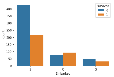
| # Embarked別の生存率
train_df["Survived"].groupby(train_df["Embarked"]).mean()
|
1
2
3
4
5
| Embarked
C 0.553571
Q 0.389610
S 0.336957
Name: Survived, dtype: float64
|
1
2
| # 要素の頻度
train_df["Embarked"].value_counts()
|
1
2
3
4
| S 644
C 168
Q 77
Name: Embarked, dtype: int64
|
1
2
| # Embarked別のSurvivedカウント
sns.countplot(data=train_df, x="Embarked",hue="Survived");
|
結果:名前,チケット番号,客室番号は,予想通りになっている.しかしながら,乗車した港は,目標変数に対して関係があることをわかった.
以上で,学習データを理解した上で,以下のように重要な説明変数を取り上げられる.
1.Placss
2.sex
3.Age
4.EmbarkedFare
5.Embarked
6.Family(SibSp+Parch)
ただし,残りのPassengerId,Name,Ticket,Cabinを除去する.
2.説明変数の加工
2.1学習とテストデータの結合
1
2
3
4
5
6
7
8
9
10
11
12
13
| # 仕切り直し
train_df = pd.read_csv("./train.csv")
test_df = pd.read_csv("./test.csv")
#不要データを除去する.
train_df = train_df.drop(['Name','Ticket', 'Cabin'], axis=1)
test_df = test_df.drop(['Name','Ticket', 'Cabin'], axis=1)
# 学習用データとテスト用データの結合
all_df = pd.concat( [train_df, test_df], sort = False ) # 並び替えナシ
# インデックス番号の振り直し (trainとtestでindexが重複するので)
all_df.reset_index( drop=True ) # 古いindexを削除
|
| PassengerId | Survived | Pclass | Sex | Age | SibSp | Parch | Fare | Embarked |
|---|
| 0 | 1 | 0.0 | 3 | male | 22.0 | 1 | 0 | 7.2500 | S |
|---|
| 1 | 2 | 1.0 | 1 | female | 38.0 | 1 | 0 | 71.2833 | C |
|---|
| 2 | 3 | 1.0 | 3 | female | 26.0 | 0 | 0 | 7.9250 | S |
|---|
| 3 | 4 | 1.0 | 1 | female | 35.0 | 1 | 0 | 53.1000 | S |
|---|
| 4 | 5 | 0.0 | 3 | male | 35.0 | 0 | 0 | 8.0500 | S |
|---|
| ... | ... | ... | ... | ... | ... | ... | ... | ... | ... |
|---|
| 1304 | 1305 | NaN | 3 | male | NaN | 0 | 0 | 8.0500 | S |
|---|
| 1305 | 1306 | NaN | 1 | female | 39.0 | 0 | 0 | 108.9000 | C |
|---|
| 1306 | 1307 | NaN | 3 | male | 38.5 | 0 | 0 | 7.2500 | S |
|---|
| 1307 | 1308 | NaN | 3 | male | NaN | 0 | 0 | 8.0500 | S |
|---|
| 1308 | 1309 | NaN | 3 | male | NaN | 1 | 1 | 22.3583 | C |
|---|
1309 rows × 9 columns
2.2カテゴリ変数の書き換え
1
2
| # ダミー変数への変換
all_df = pd.get_dummies( all_df, drop_first=True )
|
1
2
| # 欠損値の確認
all_df.isna().sum()
|
1
2
3
4
5
6
7
8
9
10
11
| PassengerId 0
Survived 418
Pclass 0
Age 263
SibSp 0
Parch 0
Fare 1
Sex_male 0
Embarked_Q 0
Embarked_S 0
dtype: int64
|
2.3欠損値の置き換え
1
2
3
| # 欠損値を平均値で埋める
all_df["Age"] = all_df["Age"].fillna( all_df["Age"].mean() )
all_df["Fare"] = all_df["Fare"].fillna( all_df["Fare"].mean() )
|
2.4データの統合
1
2
| #新たな変数Familyを作成する
all_df["Family"] = np.where( (all_df['SibSp'] == 0) & (all_df['Parch'] == 0),0,1)
|
1
2
| #新たな変数Familyを確認する
all_df['Family']
|
1
2
3
4
5
6
7
8
9
10
11
12
| 0 1
1 1
2 0
3 1
4 0
..
413 0
414 0
415 0
416 0
417 1
Name: Family, Length: 1309, dtype: int32
|
1
2
| #SibSpとParchを除去する
all_df = all_df.drop( ["SibSp", "Parch"], axis=1 )
|
| PassengerId | Survived | Pclass | Age | Fare | Sex_male | Embarked_Q | Embarked_S | Family |
|---|
| 0 | 1 | 0.0 | 3 | 22.000000 | 7.2500 | 1 | 0 | 1 | 1 |
|---|
| 1 | 2 | 1.0 | 1 | 38.000000 | 71.2833 | 0 | 0 | 0 | 1 |
|---|
| 2 | 3 | 1.0 | 3 | 26.000000 | 7.9250 | 0 | 0 | 1 | 0 |
|---|
| 3 | 4 | 1.0 | 1 | 35.000000 | 53.1000 | 0 | 0 | 1 | 1 |
|---|
| 4 | 5 | 0.0 | 3 | 35.000000 | 8.0500 | 1 | 0 | 1 | 0 |
|---|
| ... | ... | ... | ... | ... | ... | ... | ... | ... | ... |
|---|
| 413 | 1305 | NaN | 3 | 29.881138 | 8.0500 | 1 | 0 | 1 | 0 |
|---|
| 414 | 1306 | NaN | 1 | 39.000000 | 108.9000 | 0 | 0 | 0 | 0 |
|---|
| 415 | 1307 | NaN | 3 | 38.500000 | 7.2500 | 1 | 0 | 1 | 0 |
|---|
| 416 | 1308 | NaN | 3 | 29.881138 | 8.0500 | 1 | 0 | 1 | 0 |
|---|
| 417 | 1309 | NaN | 3 | 29.881138 | 22.3583 | 1 | 0 | 0 | 1 |
|---|
1309 rows × 9 columns
2.5データの分離
1
2
3
| #trainとtestに戻す
train_df_2 = all_df[:len(train_df)]
test_df_2 = all_df[len(train_df):]
|
1
2
3
4
| # 説明変数と目的変数の分離 (列を削除)
train_X = train_df_2.drop( ["Survived", "PassengerId"], axis=1 )
test_X = test_df_2.drop( ["Survived", "PassengerId"], axis=1 )
train_Y = train_df_2["Survived"]
|
1
| train_X.shape, train_Y.shape, test_X.shape
|
1
| ((891, 7), (891,), (418, 7))
|
3.機械学習
学習モデルについて,以下のようになっている.
1.決定木
2.ランダムフォレスト
3.勾配ブースティング
4.集団学習
5.スタッキング
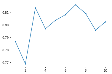
3.1決定木
1
2
3
4
5
6
7
8
9
10
11
12
| # 決定木
from sklearn.tree import DecisionTreeClassifier
from sklearn.model_selection import cross_val_score
MAX_DEPTH = 10
accuracy = np.zeros(MAX_DEPTH)
for depth in range(1, MAX_DEPTH+1):
decision_tree = DecisionTreeClassifier(max_depth = depth)
scores = cross_val_score(decision_tree,train_X,train_Y,cv=10)
accuracy[depth-1] = np.mean(scores)
plt.plot(range(1, MAX_DEPTH+1),accuracy,'.-')
|
1
| [<matplotlib.lines.Line2D at 0x1c7acaee700>]
|
1
2
3
4
| #パラメータ最適化
decision_tree = DecisionTreeClassifier(max_depth=3)#過学習を防ぐために,depth=3
decision_tree.fit(train_X, train_Y)
Y_pred_dt = decision_tree.predict(test_X)
|
1
2
3
4
| # 予測結果の出力
file = pd.read_csv("./gender_submission.csv")
file["Survived"] = Y_pred_dt.astype(int) # 整数型に変換 (少数点以下を削除)
file.to_csv("./submission_dt.csv", index=False) # indexは上書きしない
|
3.1ランダムフォレスト
1
2
3
4
5
6
7
8
9
10
11
12
13
14
15
16
17
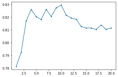
| #ランダムフォレスト
from sklearn.ensemble import RandomForestClassifier
X=train_X
Y=train_Y
MAX_DEPTH = 20
accuracy = np.zeros(MAX_DEPTH)
for depth in range(1,MAX_DEPTH+1):
model_rf = RandomForestClassifier(n_estimators = 500 ,max_depth=depth,random_state=1126)
model_rf.fit(X,Y)
model_rf.score(X, Y)
scores = cross_val_score(model_rf,X,Y,cv=20)
accuracy[depth-1] = np.mean(scores)
plt.plot(range(1, MAX_DEPTH+1),accuracy,'.-')
|
1
| [<matplotlib.lines.Line2D at 0x1c7ac1782b0>]
|
1
2
3
4
| #パラメータ最適化
model_rf = RandomForestClassifier(n_estimators = 500 ,max_depth=4,random_state=1126)
model_rf.fit(train_X,train_Y)
Y_pred_rf = model_rf.predict(test_X)
|
1
2
3
| file = pd.read_csv("./gender_submission.csv")
file["Survived"] = Y_pred_rf.astype(int) # 整数型に変換 (少数点以下を削除)
file.to_csv("./submission_rf.csv", index=False) # indexは上書きしない
|
3.3勾配ブースティング
1
2
3
4
5
6
7
8
9
10
11
12
13
14
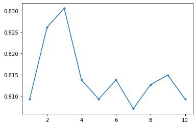
| from sklearn.ensemble import GradientBoostingClassifier
X=train_X
Y=train_Y
MAX_DEPTH = 10
accuracy = np.zeros(MAX_DEPTH)
for depth in range(1,MAX_DEPTH+1):
model_gb = GradientBoostingClassifier(n_estimators = 500 ,max_depth=depth,random_state=1234)
scores = cross_val_score(model_gb,X,Y,cv=10)
accuracy[depth-1] = np.mean(scores)
plt.plot(range(1, MAX_DEPTH+1),accuracy,'.-')
|
1
| [<matplotlib.lines.Line2D at 0x1c7ac3c4100>]
|
1
2
3
4
| #パラメータ最適化
model_gb = GradientBoostingClassifier(n_estimators = 500 ,max_depth=3,random_state=1234)
model_gb.fit(train_X,train_Y)
Y_pred_gb = model_gb.predict(test_X)
|
1
2
3
| file = pd.read_csv("./gender_submission.csv")
file["Survived"] = Y_pred_gb.astype(int) # 整数型に変換 (少数点以下を削除)
file.to_csv("./submission_gb.csv", index=False) # indexは上書きしない
|
3.4集団学習
1
2
3
4
5
6
7
8
9
10
11
12
13
14
15
16
17
18
19
20
| model1 = RandomForestClassifier( n_estimators=500,random_state=1126, max_depth = 4 )
model2 = RandomForestClassifier( n_estimators=500,random_state=9999, max_depth = 4 )
model3 = GradientBoostingClassifier( n_estimators=500,random_state=1126, max_depth = 3 )
model4 = GradientBoostingClassifier( n_estimators=500,random_state=9999, max_depth = 3 )
# 学習
model1.fit( train_X, train_Y )
model2.fit( train_X, train_Y )
model3.fit( train_X, train_Y )
model4.fit( train_X, train_Y )
# テスト
pred_test_Y1 = model1.predict( test_X )
pred_test_Y2 = model2.predict( test_X )
pred_test_Y3 = model3.predict( test_X )
pred_test_Y4 = model4.predict( test_X )
# 予測結果の多数決 (平均値)
ensemble_Y = ( pred_test_Y1 + pred_test_Y2
+ pred_test_Y3 + pred_test_Y4) / 4
|
1
2
3
4
| # 予測結果の出力
file = pd.read_csv("./gender_submission.csv")
file["Survived"] = ensemble_Y.astype(int)
file.to_csv("./submission_ENS.csv", index=False)
|
3.5スタッキング
1
2
3
4
5
6
7
8
9
10
11
12
13
14
15
16
17
18
19
20
21
22
23
24
25
26
| #スタッキング
pred_train_Y1 = model1.predict(train_X)
pred_train_Y2 = model2.predict(train_X)
pred_train_Y3 = model3.predict(train_X)
pred_train_Y4 = model4.predict(train_X)
Ens_train_Y=np.array([pred_train_Y1,pred_train_Y2,pred_train_Y3,pred_train_Y4]).T
#ここで重回帰モデルLinearClassifierをimportできないために,ほかの線形分類器を用いた.
#確率的勾配降下法SGD
from sklearn.linear_model import SGDClassifier
model_boss = SGDClassifier()
X=Ens_train_Y
Y=train_Y
model_boss.fit(X,Y)
#子分の予測
pred_test_Y1 = model1.predict(test_X)
pred_test_Y2 = model2.predict(test_X)
pred_test_Y3 = model3.predict(test_X)
pred_test_Y4 = model4.predict(test_X)
Ens_test_X = np.array([pred_test_Y1, pred_test_Y2, pred_test_Y3, pred_test_Y4 ]).T
#ボス予測
pred_test_YBoss = model_boss.predict(Ens_test_X)
|
1
2
3
| file = pd.read_csv("./gender_submission.csv")
file["Survived"] = pred_test_YBoss.astype(int) # 整数型に変換 (少数点以下を削除)
file.to_csv("./submission_STK.csv", index=False) # indexは上書きしない
|
4.Kaggle最終結果
決定木: 0.77990
ランダムフォレスト: 0.77751
勾配ブースティング: 0.75458
集団学習: 0.77511
スタッキング: 0.75598
得点最も高いのは,決定木である.
スコア
0.77990
順位
2923
ハンドルネーム
koutaku young