線形回帰モデルにおける最小二乗法(Least squares method in multiple linear regression)
Home Page:Youkoutaku
1
2
3
4
5
6
7
8
9
10
11
12
13
14
import numpy as np
import scipy as sp
import pandas as pd
from pandas import Series, DataFrame
import matplotlib.pyplot as plt
import matplotlib as mpl
import seaborn as sns
%matplotlib inline

# 小数第3位まで表示
%precision 3

# ランダムシードの固定
np.random.seed(0)
1
2
3
4
5
6
7
8
9
10
from google.colab import drive
drive.mount('/content/drive/')

# Read the CSV file from Google Drive, and the data is from course
filename = '/content/drive/My Drive/GDP.csv'

df = pd.read_csv(filename)

# Print the DataFrame
print(df)
1
2
3
4
5
6
7
8
9
10
11
12
13
14
15
Drive already mounted at /content/drive/; to attempt to forcibly remount, call drive.mount("/content/drive/", force_remount=True).
      Unnamed: 0  infant.mortality   gdp
0    Afghanistan               154  2848
1        Albania                32   863
2        Algeria                44  1531
3         Angola               124   355
4        Antigua                24  6966
..           ...               ...   ...
188     Viet.Nam                37   270
189        Yemen                80   732
190   Yugoslavia                19  1487
191       Zambia               103   382
192     Zimbabwe                68   786

[193 rows x 3 columns]
1
2
3
4
5
6
7
8
9
# get mortality
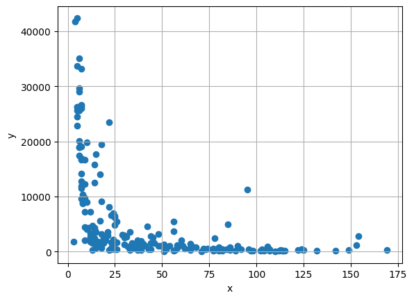
x = np.array(df.iloc[:, 1])
# get gdp
y = np.array(df.iloc[:, 2])
plt.scatter(x, y)
plt.xlabel('x')
plt.ylabel('y')
plt.grid(True)
1
2
3
4
5
6
7
8
9
10
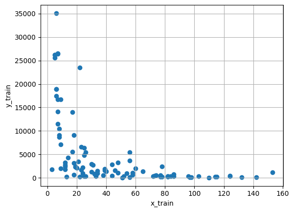
# Split the data for train and test
from sklearn.model_selection import train_test_split
x_train, x_test, y_train, y_test = train_test_split(x, y, train_size = 0.5, test_size = 0.5, random_state = 0)
#Train data
plt.scatter(x_train, y_train)
plt.xlabel('x_train')
plt.ylabel('y_train')
plt.grid(True)
1
2
3
4
5
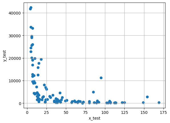
#Test data
plt.scatter(x_test, y_test)
plt.xlabel('x_test')
plt.ylabel('y_test')
plt.grid(True)
回帰モデル:
\[y=\theta_0+\theta_1\phi_1(x)+\cdots+\theta_{N-1}\phi_{N-1}(x)\]推定値: \(\hat{\theta}=(H^TH)^{-1} H^Ty\)
ただし, \(\begin{aligned}&\boldsymbol{H}=\begin{bmatrix}1&\phi_1(x_1)&...&\phi_{N-1}(x_1)\\1&\phi_1(x_2)&...&\phi_{N-1}(x_2)\\\vdots&\vdots&&\vdots\\1&\phi_1(x_M)&...&\phi_{N-1}(x_M)\end{bmatrix}\quad\boldsymbol{y}=\begin{bmatrix}y_1\\y_2\\\vdots\\y_M\end{bmatrix}\end{aligned}\)
$\phi_k(x)=x^k$として,正則化最小二乗法による推定を行う。
1
2
3
4
5
6
7
8
9
10
11
12
13
14
15
16
17
18
19
20
21
22
23
24
25
26
27
28
29
# 正則化最小二乗法で解を求める rmls(学習データ(x), 学習データ(y), 解空間の次元数N, 正規化定数ξ)
def rmls(x_train, y_train, N, gzai ):

    #行列Hの行数設定
    M=x_train.shape[0]

    #xとyをM行1列に変換
    x_train=x_train.reshape((M,1))
    y_train=y_train.reshape((M,1))

    #全ての要素が1の列ベクトルを生成
    i=np.ones((M,1))

    H=i
    for k in range(1,N):
        H=np.hstack((H,x_train**(k)))
    #print('H =', H)

    A=np.dot(H.T, H)+gzai*np.eye(N)
    B=np.dot(H.T, y_train)

    #パラメータΘの最小二乗推定値
    lss_c=np.dot(np.linalg.inv(A), B)

    #lss_cの要素を逆順に並び替え
    lss_c=np.sort(lss_c)[::-1]

    return (lss_c, M)
1
2
3
4
5
6
7
8
9
10
11
12
13
14
15
16
17
18
19
20
21
22
23
24
25
26
27
#正則化定数 0.0
#学習データと検証データでの平均二乗誤差(MSE)の表示
from sklearn.metrics import mean_squared_error
result=[]
for N in range(2,11):
    lss_c, M = rmls(x_train, y_train, N, 0.0)

    #学習データを用いてyを推定
    ys_train = np.polyval(lss_c,x_train)

    #検証データを用いてyを推定
    ys_test=np.polyval(lss_c,x_test)

    #学習データに対するyの推定値の平均二乗誤差
    train_error = mean_squared_error(y_train, ys_train)

    #検証データに対するyの推定値の平均二乗誤差
    test_error = mean_squared_error(y_test, ys_test)

    result.append([train_error, test_error])

diff = DataFrame(data=result, columns=['Training','Test'], index=[n for n in range(2,11)])

diff.plot(title='Mean Squared Error')
plt.xlabel('N')
plt.ylabel('MSE')
plt.grid(True)
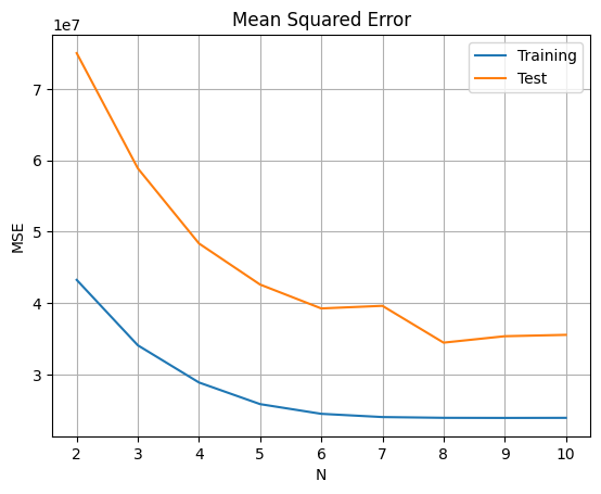
正則定数を$ξ =0.0$とした場合に,学習データと検証データでの平均二乗誤差(MSE)により,$N=8$の時に最も良い結果が得られる。
1
2
3
4
5
6
7
8
9
10
11
12
13
14
15
16
17
18
19
20
21
22
23
24
25
26
27
28
#正則化定数
#学習データと検証データでの平均二乗誤差(MSE)の表示
from sklearn.metrics import mean_squared_error
result=[]
N = 8
for gzai in range(0, 10):
    lss_c, M = rmls(x_train, y_train, N, gzai)

    #学習データを用いてyを推定
    ys_train = np.polyval(lss_c,x_train)

    #検証データを用いてyを推定
    ys_test=np.polyval(lss_c,x_test)

    #学習データに対するyの推定値の平均二乗誤差
    train_error = mean_squared_error(y_train, ys_train)

    #検証データに対するyの推定値の平均二乗誤差
    test_error = mean_squared_error(y_test, ys_test)

    result.append([train_error, test_error])

diff = DataFrame(data=result, columns=['Training','Test'], index=[n for n in range(0, 10)])

diff.plot(title='Mean Squared Error')
plt.xlabel('gzai')
plt.ylabel('MSE')
plt.grid(True)
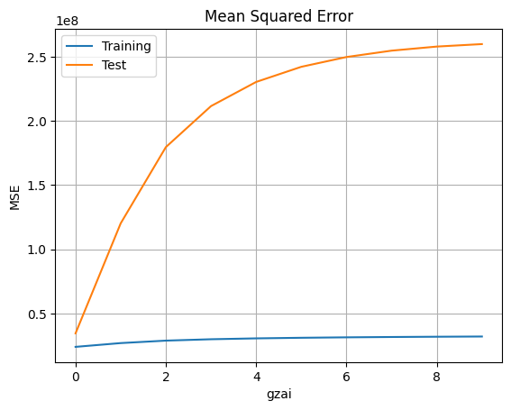
回帰次数が$N=8$とした場合に,学習データと検証データでの平均二乗誤差(MSE)により,正則化定数が$\xi=0.0$の時に最も良い結果が得られる。正則化定数が大きくなると,過学習になる。
1
2
3
4
5
6
7
8
9
10
11
12
13
14
15
16
17
18
19
20
21
22
23
24
25
# 回帰次数
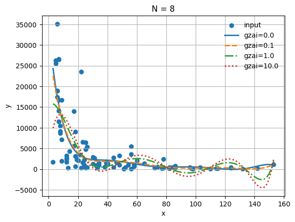
N = 8
#データプロット
plt.scatter(x_train, y_train,label='input')
#正則化パラメタのリスト
gzai=np.array([0, 0.1, 1, 10])
#プロットのラインスタイル
ls=['-', '--', '-.', ':']
#正則化最小二乗法による推定
for i in np.arange(gzai.size):
lss_c, M =rmls(x_train, y_train, N, gzai[i])
xs = np.linspace(np.min(x_train),np.max(x_train),M)
ys = np.polyval(lss_c,xs)
plt.plot(xs, ys, label='gzai='+str(round(gzai[i], 3)), ls=ls[i], lw=2)
#結果の表示
plt.title('N = %d' % (N))
plt.xlabel('x')
plt.ylabel('y')
plt.legend(loc='best',frameon=False)
plt.grid(True)
1
2
# 推定パラメータ
print(lss_c)
1
2
3
4
5
6
7
8
[[ 1.430e-08]
 [-7.813e-06]
 [ 1.692e-03]
 [-1.841e-01]
 [ 1.048e+01]
 [-2.911e+02]
 [ 2.971e+03]
 [ 3.486e+03]]
最も良い回帰モデル: \(y=1.430\times10^{-8}x-7.813\times10^{-6}x^2+1.692\times10^{-3}x^3-1.841\times10^{-1}x^4+1.048\times10^{1}x^5-2.911\times10^{2}x^6+2.971\times10^{3}x^7+3.486\times10^{3}x^8\)
This post is licensed under CC BY 4.0 by the author.