LQR for tracking

Problem Formulation

Consider a discrete-time linear system, the state-space equation is as

\[x_{[k+1]}=f(x_{[k]},u_{[k]})=Ax_{[k]}+Bu_{[k]}\]

where $x_{[k]}\in\mathbb{R}^n,u_{[k]}\in\mathbb{R}^p$ are system state and input, $A_{[k]}\in\mathbb{R}^{n\times n}$, $B_{[k]}\in\mathbb{R}^{n\times p}$ are state matrices for system.

The tracking reference is as

\[x^r_{[k+1]}=A_rx^r_{[k]}\]

Define the tracking error as

\[e_{[k]}=x_{[k]}-x^r_{[k]}\]

Define the increase of input as

\[\Delta u_{[k]}=u_{[k]}-u_{[k-1]}\implies u_{[k]}=\Delta u_{[k]}+u_{[k-1]}\]

Then, the state-space equation is rewrite as

\[x_{[k+1]}=Ax_{[k]}+B(\Delta u_{[k]}-u_{[k-1]})\]

Define the augmented states as

\[\begin{bmatrix} x_{[k+1]}\\x^r_{[k+1]}\\u_{[k]} \end{bmatrix} =\begin{bmatrix} A &0_{n\times n} &B\\0_{n\times n} &A_r &0_{n\times p}\\ 0_{p\times n} &0_{p\times n} &I_{p\times p} \end{bmatrix}\begin{bmatrix} x_{[k]}\\ x^r_{[k]} \\ u_{[k-1]} \end{bmatrix}+\begin{bmatrix} B\\0_{n\times p} \\ I_{p\times p} \end{bmatrix}\Delta u_{[k]}\]

where

\[z_{[k]}:=\begin{bmatrix} x_{[k]}\\ x^r_{[k]} \\ u_{[k-1]} \end{bmatrix}, A_z:=\begin{bmatrix} A &0_{n\times n} &B\\0_{n\times n} &A_r &0_{n\times p}\\ 0_{p\times n} &0_{p\times n} &I_{p\times p} \end{bmatrix}, B_z:=\begin{bmatrix} B\\0_{n\times p}\\I_{p\times p} \end{bmatrix}\]

Then, we have

\[z_{[k+1]}=A_zz_{[k]}+B_z\Delta u_{[k]}\] \[e_{[k]}=[I_{n\times n}\;-I_{n\times n}\;0_{n\times p}]z_{[k]}=C_zz_{[k]}\]

Define the quadratic performance function as

\[J=h\left(e_{[N]}\right)+\sum_{k=0}^{N-1}g\left(e_{[k]},u_{[k]}\right)\]

where

\[\begin{aligned}&h\left(e_{[N]}\right)=\frac{1}{2}e_{[N]}^{T}Se_{[N]}\\&g\left(e_{[k]},u_{[k]}\right)=\frac{1}{2}[e_{[k]}^{T}Qe_{[k]}+\Delta u_{[k]}^{T}R\Delta u_{[k]}]\end{aligned}\]

---

Solving

\[J= \frac{1}{2}e_{[N]}^{T}Se_{[N]} +\frac{1}{2}\sum_{k=0}^{N-1}[e_{[k]}^{T}Qe_{[k]}+\Delta u_{[k]}^{T}R\Delta u_{[k]}]\] \[J= \frac{1}{2}(C_zz_{[N]}) ^{T}S(C_zz_{[N]}) +\frac{1}{2}\sum_{k=0}^{N-1}[(C_zz_{[k]})^{T}QC_zz_{[k]}+\Delta u_{[k]}^{T}R\Delta u_{[k]}]\] \[J= \frac{1}{2}z_{[N]}^{T}(C_z^TSC_z)z_{[N]} +\frac{1}{2}\sum_{k=0}^{N-1}[z_{[k]}^T(C_z^{T}QC_z)z_{[k]}+\Delta u_{[k]}^{T}R\Delta u_{[k]}]\]

• $S^z=C_z^TSC_z$
• $Q^z=C_z^TQC_z$

\[J= \frac{1}{2}z_{[N]}^{T}(S^z)z_{[N]} +\frac{1}{2}\sum_{k=0}^{N-1}[z_{[k]}^TQ^zz_{[k]}+\Delta u_{[k]}^{T}R\Delta u_{[k]}]\]

According to LQR Gain ($x \to z$), the optimal increase of input:

\[\Delta u^\ast_{[N-k]}=-F_{[N-k]}z_{[N-k]}\]

where

\[F_{[N-k]}=(B^{T}P_{[k-1]}B+R)^{-1}B^{T}P_{[k-1]}A\]

Notice that the increase of input is optimized.

\[P_{[k]}=(A-BF_{[N-k]})^TP_{[k-1]}(A-BF_{[N-k]})+F_{[N-k]}^TRF_{[N-k]}+Q\] \[P_{[0]}=S^z\implies P_{[1]}, \Delta u^\ast_{[N-1]}\implies \cdots P_{[k]}, \Delta u^\ast_{[N-k]} \cdots \implies P_{[N]}, \Delta u^\ast_{[0]}\]

The optimal input is

\[u_{[k]}^\ast=\Delta u^\ast_{[k]}+u^\ast_{[k-1]}\]

---

Simulation

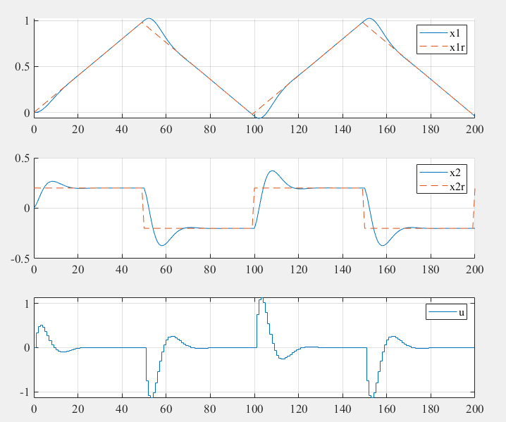
Consider a simple 2nd-order system:

\[\begin{bmatrix} \dot x_1 \\ \dot x_2 \end{bmatrix}=\begin{bmatrix} 0 &1\\ 0 &0 \end{bmatrix}\begin{bmatrix} x_1 \\ x_2 \end{bmatrix}+\begin{bmatrix}0\\ 1 \end{bmatrix}u(t)\] \[x^r(0)=\begin{bmatrix} 0\\ 0.2\\ \end{bmatrix}\]

• weight matrix

\[Q=\begin{bmatrix} 1 & 0 \\ 0 & 1 \end{bmatrix}, S=\begin{bmatrix} 1 & 0 \\ 0 & 1 \end{bmatrix}, R=0.1\]

%% LQR for Tracking problem
%-----------------------------------------------%
% Youkoutaku:  https://youkoutaku.github.io/
% Date: 2024/01/16
% Description: LQR for tracking problem. The reference signal is time-varying.
%-----------------------------------------------%
% Augmented_System_Input.m is a function to create the augmented system for the increase of input.
% [Az,Bz,Qz,Rz,Sz] = Augmented_System_Input(A,B,Q,R,S,Ar) creates the augmented system for the increase of input.

clear;
close all;
clc;
set(0, 'DefaultAxesFontName', 'Times New Roman')
set(0, 'DefaultAxesFontSize', 14)
  
%% System Model
A = [0 1; 0 0];
n = size(A, 1);
B = [0; 1];
p = size(B, 2);
C = [1 0; 0 1];
D = [0; 0];

%% System Setting
Ts = 0.1; %Sample time
sys_d = c2d(ss(A, B, C, D), Ts); %discretization of continuous time system
A = sys_d.a; %discretized system matrix A
B = sys_d.b; %discretized input matrix B

%% Weight matrix
Q = [1 0; 0 1]; %R^(n x n) tracking error weight
S = [1 0; 0 1]; %R^(n x n) reference weight
R = 0.1; %R^(p x p) input weight

%% Initial state
x0 = [0; 0];
x = x0;

%input init
u0 = 0;
u = u0;

%% Reference Signal
xr = [0; 0.2];
Ar = c2d(ss( [0 1; 0 0],[0; 0],[1,0; 0,1],[0; 0]),Ts).A; % Augmented matrix
z = [x; xr; u];

%% Augmented System
[Az, Bz, Qz, Rz, Sz] = Augmented_System_Input(A, B, Q, R, S, Ar);

%% LQR Gain
[F] = LQR(Az, Bz, Qz, Rz, Sz);

%% Simulation
k_steps = 200;
x_h = zeros(n, k_steps);
x_h(:, 1) = x;
u_h = zeros(p, k_steps);
u_h(:, 1) = u;
xr_h = zeros(n,k_steps);
xr_h(:, 1) = xr;

for k = 1:k_steps
    % Reference Signal
    %xr = [sin(0.05 * k); 0.05*cos(0.05 * k)];
    if (k==50)
        xr = [xr(1) ; -0.2];
    elseif (k==100)
        xr = [xr(1) ; 0.2];
    elseif (k==150)
        xr = [xr(1) ; -0.2];
    elseif (k==200)
        xr = [xr(1) ; 0.2];
    end

    % Increase of input
    Delta_u = -F * z;

    % Input
    u = Delta_u + u;

    % Update System
    x = A * x + B * u;
    xr = Ar * xr;
    z = [x; xr; u];

    % Save data
    x_h(:, k + 1) = x;
    u_h(:, k + 1) = u;
    xr_h(:, k + 1) = xr;
end

%% figure
subplot (3, 1, 1);
plot (0:length(x_h)-1,x_h(1,:));
hold;
plot (0:length(xr_h)-1,xr_h(1,:),'--');
hold off;
legend("x1","x1_r");
xlabel("step");
ylabel("position");
xlim([0 k_steps]);
grid on;

subplot (3, 1, 2);
plot (0:length(x_h)-1,x_h(2,:));
hold;
plot (0:length(xr_h)-1,xr_h(2,:),'--');
hold off;
legend("x2","x2_r");
xlabel("step");
ylabel("velocity");
xlim([0 k_steps]);
grid on;

subplot (3, 1, 3);
hold;
stairs (0:length(u_h)-1,u_h(1,:));
hold off;
legend("u");
xlabel("step");
ylabel("input");
xlim([0 k_steps]);
grid on;

LQR, a feedback control, selects the optimal feedback gain by dynamic programming. However, it can not solve the optimal problem for constraint.

---

Reference

• Chris Mavrogiannis. lec15_lqr
• 王天威. 控制之美(卷2). 清华大学出版社. 2023.