LQR for Discrete-time System

Posted May 30, 2024

LQR

By Youkoutaku 5 min read

We discuss a typical problem: for the linear system, the performance function is in quadratic form, and the control goal is to stabilize the state at 0 (regulation problem). Then, its’ controllers are called linear quadratic regulators (LQR).

Problem Formulation

Consider a discrete-time linear system, the state-space equation is as

\[x_{[k+1]}=f(x_{[k]},u_{[k]})=A_{[k]}x_{[k]}+B_{[k]}u_{[k]}\]

where $x_{[k]}\in\mathbb{R}^n,u_{[k]}\in\mathbb{R}^p$ are system state and input, $A_{[k]}\in\mathbb{R}^{n\times n}$, $B_{[k]}\in\mathbb{R}^{n\times p}$ are state matrices for system.

Define the quadratic performance function as

\[J=h\left(x_{[N]}\right)+\sum_{k=0}^{N-1}g\left(x_{[k]},u_{[k]}\right)\]

where

\[\begin{aligned}&h\left(x_{[N]}\right)=\frac{1}{2}x_{[N]}^TSx_{[N]}\\&g\left(x_{[k]},u_{[k]}\right)=\frac{1}{2}\sum_{k=0}^{N-1}[x_{[k]}^TQ_{[k]}x_{[k]}+u_{[k]}^TR_{[k]}u_{[k]}]\end{aligned}\]

and the constant $\frac{1}{2}$ is used to simplify calculations when taking derivatives.

$x_{[N]}$ is the system state for terminal time $N$. $S,Q_{[N]}\in\mathbb{R}^{n\times n}$ are symmetrically positive semi definite matrix as the weight matrix for terminal cost and running cost. $R_{[k]}\in\mathbb{R}^{p\times p}$ is symmetrically positive definite matrix as the weight matrix for input cost.

\[\begin{aligned}&S=\begin{bmatrix}s_{1}&\cdots&0\\\vdots&\ddots&\vdots\\0&\cdots&s_{n}\end{bmatrix},\quad s_{1},s_{2},\cdots,s_{n}\geqslant0\\&Q_{[k]}=\begin{bmatrix}q_{1_{[k]}}&\cdots&0\\\vdots&\ddots&\vdots\\0&\cdots&q_{n_{[k]}}\end{bmatrix},\quad q_{1_{[k]}},q_{2_{[k]}},\cdots,q_{n_{[k]}}\geqslant0\\&R_{[k]}=\begin{bmatrix}r_{1_{[k]}}&\cdots&0\\\vdots&\ddots&\vdots\\0&\cdots&r_{p_{[k]}}\end{bmatrix},\quad r_{1_{[k]}},r_{2_{[k]}},\cdots,r_{p_{[k]}}>0\end{aligned}\]

Backward multi stages

$k=N \to k=N$

The performance function for $N\to N$:

\[J_{N\to N}(x_{[N]})=\frac{1}{2}x_{[N]}^TSx_{[N]}\]

And it also is the optimal cost for $N\to N$.

\[J_{N\to N}^*(x_{[N]})=\frac{1}{2}x_{[N]}^TP_{[0]}x_{[N]}\]

Define $P_{[0]}\triangleq S$.

$k=N-1 \to k=N$

The cost to go:

\[\begin{aligned} J_{N-1+N}(x_{[N-1]},x_{[N]},u_{[N-1]})=\frac{1}{2}x_{[N]}^TSx_{[N]}+\\\frac{1}{2}(x_{[N-1]}^TQ_{[N-1]}x_{[N-1]}+u_{[N-1]}^TR_{[N-1]}u_{[N-1]}) \end{aligned}\]

According to $x_{[N]}=A_{[N-1]}x_{[N-1]}+B_{[N-1]}u_{[N-1]}$, we can obtain the following cost to go only relying on $x_{[N-1]}$ and $u_{[N-1]}$,

\[\begin{aligned} J_{N-1\to N}(x_{[N-1]}, u_{[N-1]})&=\boxed{\frac{1}{2}[A_{[N-1]}x_{[N-1]}+B_{[N-1]}u_{[N-1]}]^TP_{[0]}[A_{[N-1]}x_{[N-1]}+B_{[N-1]}u_{[N-1]}]}\\+&\boxed{\frac{1}{2}(x_{[N-1]}^TQ_{[N-1]}x_{[N-1]}+u_{[N-1]}^TR_{[N-1]}u_{[N-1]})} \end{aligned}\]

Then, To minimize the cost to go, we can calculate the derivatives to obtain the optimal control input.

\[\frac{\partial J_{N-1\to N}(x_{[N-1]},u_{[N-1]})}{\partial u_{[N-1]}}=0\]

Define $y(u_{[N-1]})$ ,making the following equation.
\[\begin{aligned}&\boxed{\frac{1}{2}[A_{[N-1]}x_{[N-1]}+B_{[N-1]}u_{[N-1]}]^TP_{[0]}[A_{[N-1]}x_{[N-1]}+B_{[N-1]}u_{[N-1]}]}\\&=\frac{1}{2}y(u_{[N-1]})^TP_{[0]}y(u_{[N-1]})\end{aligned}\] \[\begin{aligned} &\frac{\partial\left(\frac{1}{2}y\left(u_{[N-1]}\right)^{T}P_{[0]}y\left(u_{[N-1]}\right)\right)}{\partial u_{[N-1]}}=\frac{\partial y(u_{[N-1]})}{\partial u_{[N-1]}}\frac{\partial \frac{1}{2}y(u_{[N-1]})^{T}P_{[0]}y(u_{[N-1]})}{\partial y(u_{[N-1]})} \end{aligned}\] \[\frac{\partial y(u_{[N-1]})}{\partial u_{[N-1]}}=\frac{\partial(A_{[N-1]}x_{[N-1]}+B_{[N-1]}u_{[N-1]})}{\partial u_{[N-1]}}=B_{[N-1]}^{T}\] \[\frac{\partial \frac{1}{2}y(u_{[N-1]})^TP_{[0]}y(u_{[N-1]})}{\partial y(u_{[N-1]})}=P_{[0]}y(u_{[N-1]})\] \[\frac{\partial \boxed{\frac{1}{2}(x_{[N-1]}^TQ_{[N-1]}x_{[N-1]}+u_{[N-1]}^TR_{[N-1]}u_{[N-1]})}}{\partial u_{[N-1]}}=R_{[N-1]}u_{[N-1]}\]

Therefor, we have

\[\frac{\partial J_{N-1\to N}(x_{[N-1]},u_{[N-1]})}{\partial u_{[N-1]}}=B_{[N-1]}^{T}P_{[0]}\left[A_{[N-1]}x_{[N-1]}+B_{[N-1]}u_{[N-1]}\right]+R_{[N-1]}u_{[N-1]}\]

In order to minimize cost to go, we make it equal to 0.

\[B_{[N-1]}^{T}P_{[0]}\left[A_{[N-1]}x_{[N-1]}+B_{[N-1]}u_{[N-1]}\right]+R_{[N-1]}u_{[N-1]}=0\]

\[B_{[N-1]}^{T}P_{[0]}A_{[N-1]}x_{[N-1]}+B_{[N-1]}^{T}P_{[0]}B_{[N-1]}u_{[N-1]}+R_{[N-1]}u_{[N-1]}=0\] \[u_{[N-1]}=-\left(B_{[N-1]}^{T}P_{[0]}B_{[N-1]}+R_{[N-1]}\right)^{-1}B_{[N-1]}^{T}P_{[0]}A_{[N-1]}x_{[N-1]}\]

Then, we can obtain the following optimal control input

\[u_{[N-1]}^*=-F_{[N-1]}x_{[N-1]}\]

where

\[F_{[N-1]}=(B_{[N-1]}^TP_{[0]}B_{[N-1]}+R_{[N-1]})^{-1}B_{[N-1]}^TP_{[0]}A_{[N-1]}.\]

To verify the minimum, we need the second derivative for cost to go.

\[\begin{aligned} &\frac{\partial^{2}\left(J_{N-1\to N}\left(x_{[N-1]},u_{[N-1]}\right)\right)}{\partial u_{[N-1]}^{2}} \\ &=\frac{\partial[B_{[N-1]}^TP_{[0]}(A_{[N-1]}x_{[N-1]}+B_{[N-1]}u_{[N-1]})+R_{[N-1]}u_{[N-1]}]}{\partial u_{[N-1]}} \\ &=B_{[N-1]}^TP_{[0]}B_{[N-1]}+R_{[N-1]}>0 \end{aligned}\]

Therefor, The $J_{N-1\to N}\left(x_{[N-1]},u_{[N-1]}\right)$ has a minimum for $u_{[N-1]}=u^*_{[N-1]}$ .

The optimal cost to go:

\[\begin{aligned} J_{N-1\to N}^*(x_{[N-1]})=&\frac{1}{2}[A_{[N-1]}x_{[N-1]}-B_{[N-1]}F_{[N-1]}x_{[N-1]}]^TP_{[0]}[A_{[N-1]}x_{[N-1]}-B_{[N-1]}F_{[N-1]}x_{[N-1]}]\\&+\frac{1}{2}\Big[x_{[N-1]}^{T}Q_{[N-1]}x_{[N-1]}+ (-F_{[N-1]}x_{[N-1]})^TR_{[N-1]}(-F_{[N-1]}x_{[N-1]})\Big] \end{aligned}\]

$\implies$

\[J_{N-1\to N}^{*}(x_{[N-1]})=\frac{1}{2}x_{[N-1]}^TP_{[1]}x_{[N-1]}\]

where

\[P_{[1]}\triangleq (A_{[N-1]}-B_{[N-1]}F_{[N-1]})^TP_{[0]}(A_{[N-1]}-B_{[N-1]}F_{[N-1]})+F_{[N-1]}^TR_{[N-1]}F_{[N-1]}+Q_{[N-1]}.\]

$k=N-2 \to k=N$

The cost to go:

\[\begin{aligned} J_{N-2\to N}(x_{[N-2]},x_{[N-1]},u_{[N-1]},u_{[N-2]})& = \frac{1}{2}x_{[N]}{}^TSx_{[N]}\\ &+\frac{1}{2}(x_{[N-1]}^TQ_{[N-1]}x_{[N-1]}+ u_{[N-1]}^TR_{[N-1]}u_{[N-1]})\\&+\frac12(x_{[N-2]}^TQ_{[N-2]}x_{[N-2]}+u_{[N-2]}^TR_{[N-2]}u_{[N-2]}) \\ &=J_{N-1\to N}(x_{[N-1]},u_{[N-1]})\\&+\frac{1}{2}(x_{[N-2]}^TQ_{[N-2]}x_{[N-2]}+u_{[N-2]}^TR_{[N-2]}u_{[N-2]}) \end{aligned}\]

According to Bellman optimal theory, we have the optimal cost to go based on the optimal cost to go for $N-1\to N$ as

\[\begin{aligned} J_{N-2\to N}^{*}(x_{[N-2]})& =\min_{u_{[N-1]}}\Big(J_{N-1\to N}^{*}(x_{[N-1]})+ \\ &\frac12(x_{[N-2]}^TQ_{[N-2]}x_{[N-2]}+u_{[N-2]}^TR_{[N-2]}u_{[N-2]})\Big) \\ &=\min_{u_{[N-1]}}\Big(\frac{1}{2}x_{[N-1]}^TP_{[1]}x_{[N-1]}+ \\ &\frac{1}{2}(x_{[N-2]}^TQ_{[N-2]}x_{[N-2]}+u_{[N-2]}^TR_{[N-2]}u_{[N-2]})\Big)\end{aligned}\]

According to $x_{[N-1]}=A_{[N-2]}x_{[N-2]}+B_{[N-2]}u_{[N-2]}$, we can obtain the following cost to go only relying on $x_{[N-2]}$ and $u_{[N-2]}$,

\[\begin{aligned} J_{N-2\to N}^{*}(x_{[N-2]})&=\min_{u_{[N-1]}}\Big(\frac{1}{2}\left[A_{[N-2]}x_{[N-2]}+B_{[N-2]}u_{[N-2]}\right]^TP_{[1]}\left[A_{[N-2]}x_{[N-2]}+B_{[N-2]}u_{[N-2]}\right]\\ &+ \frac{1}{2}(x_{[N-2]}^TQ_{[N-2]}x_{[N-2]}+u_{[N-2]}^TR_{[N-2]}u_{[N-2]})\Big)\end{aligned}\]

Then, To minimize the cost to go, we can calculate the derivatives to obtain the optimal control input.

\[\frac{\partial J_{N-2\to N}(x_{[N-1]},u_{[N-1]})}{\partial u_{[N-2]}}=0\]

Similar to $N-1\to N$, we can obtain the following equation.

\[B_{[N-2]}^{T}P_{[1]}\left[A_{[N-2]}x_{[N-2]}+B_{[N-2]}u_{[N-2]}\right]+R_{[N-2]}u_{[N-2]}=0\]

Therefor, the optimal control input is

\[u^*_{[N-2]}=-F_{[N-2]}x_{[N-2]}\]

where

\[F_{[N-2]}=(B_{[N-2]}^TP_{[1]}B_{[N-2]}+R_{[N-2]})^{-1}B_{[N-2]}^TP_{[1]}A_{[N-2]}.\]

The optimal cost to go:

\[J_{N-2\to N}^{*}(x_{[N-2]})=\frac{1}{2}x_{[N-2]}^{T}P_{[2]}x_{[N-2]}\]

where

\[P_{[2]}\triangleq (A_{[N-2]}-B_{[N-2]}F_{[N-2]})^TP_{[1]}(A_{[N-2]}-B_{[N-2]}F_{[N-2]})+F_{[N-2]}^TR_{[N-2]}F_{[N-2]}+Q_{[N-2]}.\]

$N-k \to N$

The optimal control input:

\[u^*_{[N-k]}=-F_{[N-k]}x_{[N-k]}\]

where

\[F_{[N-k]}=(B_{[N-k]}^TP_{[k-1]}B_{[N-k]}+R_{[N-k]})^{-1}B_{[N-k]}^TP_{[k-1]}A_{[N-k]}.\]

The optimal cost to go:

\[J_{N-k\to N}^{*}(x_{[N-k]})=\frac{1}{2}x_{[N-k]}^{ T}P_{[k]}x_{[N-k]}\]

where

\[P_{[k]}\triangleq (A_{[N-k]}-B_{[N-k]}F_{[N-k]})^TP_{[k-1]}(A_{[N-k]}-B_{[N-k]}F_{[N-k]})+F_{[N-k]}^TR_{[N-k]}F_{[N-k]}+Q_{[N-k]}.\]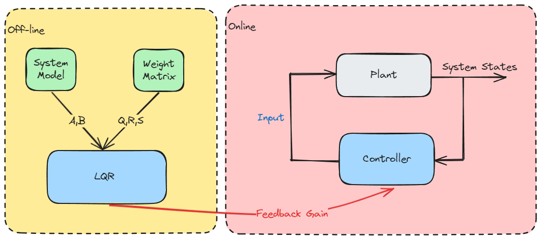

The LQR controller is a feedback control where the $F_{[N-k]}$ is the feedback gain. In fact, by minimizing the cost function, we obtain the optimal feedback gain to calculate the control input.

If the system is linear time-invariant and fully controllable, we have a constant feedback gain $F$.

\[N\to\infty\implies F_{[N-k]}\to F\]

Therefor, the solving for optimal control can off-line.

\[P_{[0]}=S\implies P_{[1]}, u^*_{[N-1]}\implies \cdots P_{[k]}, u^*_{[N-k]} \cdots \implies P_{[N]}, u^*_{[0]}\]

In real-time system, we use the optimal control input $u^*_{[0]},\cdots,u^*_{[N-k]},\cdots,u^*_{[N-1]}$ for the system states $x_{[0]}\implies \cdots x_{[N-k]} \cdots \implies x_{[N]}$.

Code

Matlab

  
function [F] = LQR(A,B,Q,R,S)
% P_[0]
P0 = S;
% Maximum number of step
max_iter = 200;
% Convergence difference
mini = 1e-3;
% Initial value
P_k_min_1 = P0;
diff = Inf;
F_N_min_k = Inf;
k = 1;
while diff > mini
	% F_[N-(k-1)]
	F_N_min_k_pre = F_N_min_k;
	% F_[N-k]
	F_N_min_k = (R+B'*P_k_min_1*B)\B'*P_k_min_1*A;
	% P_[k]
	P_k = (A-B*F_N_min_k)'*P_k_min_1*(A-B*F_N_min_k)+(F_N_min_k)'*R*(F_N_min_k)+Q;
	% P_[k-1]
	P_k_min_1 = P_k;
	% F_[N-k] - F_[N-(k-1)]
	diff = abs(max(F_N_min_k - F_N_min_k_pre));
	k = k + 1;
	if k > max_iter
		error('Maximum Number of Iterations Exceeded');
	end
end
fprintf('No. of Interation is %d \n', k);
F=F_N_min_k;
end

Python

  
def lqr(A, B, Q, R, S):
    # P_[0]
    P0 = S
    # Maximum number of steps
    max_iter = 200
    # Convergence difference
    mini = 1e-3
    # Initial value
    P_k_min_1 = P0
    diff = np.inf
    F_N_min_k = np.inf
    k = 1
    while diff > mini:
        # F_[N-(k-1)]
        F_N_min_k_pre = F_N_min_k
        # F_[N-k]
        F_N_min_k = np.linalg.inv(R + B.T @ P_k_min_1 @ B) @ B.T @ P_k_min_1 @ A
        # P_[k]
        P_k = (A - B @ F_N_min_k).T @ P_k_min_1 @ (A - B @ F_N_min_k) + F_N_min_k.T @ R @ F_N_min_k + Q
        # P_[k-1]
        P_k_min_1 = P_k
        # F_[N-k] - F_[N-(k-1)]
        diff = np.max(np.abs(F_N_min_k - F_N_min_k_pre))
        k += 1
        if k > max_iter:
            raise ValueError('Maximum Number of Iterations Exceeded')
    print(f'No. of Iterations is {k}')
    return F_N_min_k

Reference

Optimal Control by DR_CAN
王天威. 控制之美(卷2). 清华大学出版社. 2023.
Rakovic, S. V., & Levine, W. S. Handbook of model predictive control. 2018.

Model Predict Control, LQR

This post is licensed under CC BY 4.0 by the author.

Problem Formulation

Backward multi stages

$k=N \to k=N$

$k=N-1 \to k=N$

$k=N-2 \to k=N$

$N-k \to N$

Code

Matlab

Python

Reference

Trending Tags