Dynamic Programming and Bellman Optimal Theory

Posted May 23, 2024 Updated Jul 16, 2024

By Youkoutaku 7 min read

Bellman optimal theory

An optimal policy has the property that whatever the initial state and initial decision are, the remaining decisions must constitute an optimal policy with regard to the state resulting from the first decision.

whatever the initial state and initial decision.
the remaining decisions must constitute an optimal policy.

The dynamic programming is a method for Bellman optimal control.

Numerical Methods for optimal control

State space

\[\dot x(t)=\begin{bmatrix}0 & 1\\ 0 &0\end{bmatrix}x+\begin{bmatrix}0\\ 1\end{bmatrix}u\] \[x(t)=\begin{bmatrix}x_1(t)\\ x_2(t)\end{bmatrix}=\begin{bmatrix}h(t)\\ v(t)\end{bmatrix}\]

$h(t)$: the position of drone
$v(t)$: the velocity of drone
Initial state

\[x_0=\begin{bmatrix}0\\0\end{bmatrix}\]

Reference

\[x_d=\begin{bmatrix}10\\0\end{bmatrix}\]

Constraint condition

\[-3 \text{m/s}^2 \le u \le 2 \text{m/s}^2\] \[0 \text{m/s} \le x_2 \le 3 \text{m/s}\]

Cost function( minimum time):

\[J=\int^{t_f}_{t_0}dt=t_f-t_0\]

State space discretization

Markov chain

Divide $x_1$ into 5 zones and $x_2$ into 3 zones. We obtain 6 nodes for $x_1$ and 4 nodes for $x_2$.

The optimization task can be explained as finding the trajectory from the initial position to the target position, satisfying the constraints, and keeping the cost function to a minimum.

Solutions

Brute Force Search (Exhaustive method)
- Huge computation.
- calculate the cost function for every state.
Dynamic Programming(By Backward multi stages)
- Less computation.
- Starting from the end state, calculate the cost function for each optimal state in reverse direction.

The main idea of dynamic programming is to avoid redundant calculations by storing the results of subproblems. So that they can be directly used when needed, thus improving efficiency.

Brute Force Search

$n_{x_1}=length(x_1)=6$
$n_{x_2}=length(x_2)=4$

Calculate times for all of the paths:

\[n_{x_2}^{(n_{x_1}-2)}=4^{(6-2)}=256\]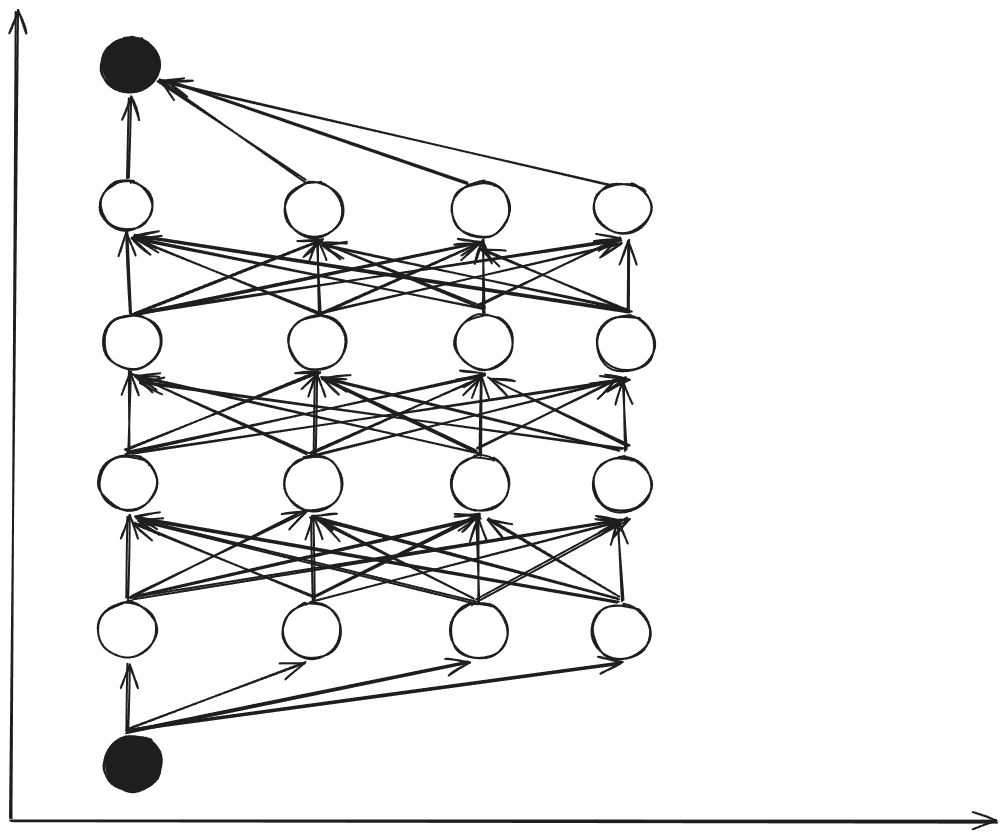

Backward multi stages

$n_{x_1}:k=1,2,3,4,5,6$

The velocity among nodes

\[{v_{avg}}_{[k\to k+1]}={x_2}_{[k\to k+1]}=\frac{1}{2}(x_{[k]}+{x_2}_{[k+1]})\]

The time from $k$ to $k+1$

\[\Delta t_{[k\to k+1]}=\frac{\Delta x_1}{ {v_{avg}}_{[k\to k+1]} }=\frac{2\Delta x_1}{ {x_2}_{[k]}+{x_2}_{[k+1]}}\]

The input form $k$ to $k+1$

\[u_{[k\to k+1]}=\frac{v_{[k+1]}-v_{[k]}}{\Delta t_{[k\to k+1]}}=\frac{ {x_2^2}_{[k+1]}+{x_2^2}_{[k]}}{2\Delta x_1}\]

$5\to6$

$k=6: x_{[6]}=[10\;0]^T$

\[k=5: x_{[5_1]}=[8\;0]^T, x_{[5_2]}=[8\;1]^T, x_{[5_3]}=[8\;2]^T, x_{[5_4]}=[8\;3]^T\] \[\Delta t_{[5_1\rightarrow6]}=\frac{2\Delta x_{1}}{x_{2_{[5_1]}}+x_{2_{[6]}}}=\frac{4}{0+0}=\infty\] \[u_{[5_1\rightarrow6]}=\frac{x_{2_{[6]}}^{2}-x_{2_{[5_1]}}^{2}}{2\Delta x_{1}}=\frac{0-0}{4}=0\] \[\Delta t_{[5_{2}\to6]}= \frac{2\Delta x_{1}}{x_{2_{[5_2]}}+x_{2_{[6]}}}=\frac{4}{1+0}=4\] \[u_{[5_2\to6]}= \frac{x_{2_{[6]}}^{2}-x_{2_{[5_2]}}^{2}}{2\Delta x_{1}}=\frac{0-1}{4}=-\frac{1}{4}\] \[\Delta t_{[5_3\to6]}=\frac{2\Delta x_{1}}{x_{2_{[5_3]}}+x_{2_{[6]}}}=\frac{4}{2+0}=2\] \[u_{[5_3\to6]}= \frac{x_{2_{[6]}}^{2}-x_{2_{[5_3]}}^{2}}{2\Delta x_{1}}=\frac{0-4}{4}=-1\] \[\Delta t_{[5_4\to6]}=\frac{2\Delta x_{1}}{x_{2_{[5_4]}}+x_{2_{[6]}}}=\frac{4}{3+0}=\frac{4}{3}\] \[u_{[5_4\to6]}= \frac{x_{2_{[6]}}^{2}-x_{2_{[5_4]}}^{2}}{2\Delta x_{1}}=\frac{0-9}{4}=- \frac{9}{4}\]

Then, We obtain the cost ot go $J^*$, means the minimum cost from a node to end node.

\[\begin{aligned} J_{[5_1\to6]}^*&=\Delta t_{[5_1\to6]}=\infty \\ J_{[5_2\to6]}^*&=\Delta t_{[5_2\to6]}=4\\ J_{[5_3\to6]}^{*}&=\Delta t_{[5_3\to6]}=2\\ J_{[5_4\to6]}^{*}&=\Delta t_{[5_4\to6]}=\frac{4}{3} \end{aligned}\] \[\begin{aligned} u_{[5_1]}^*&=u_{[5_1\to6]}=0 \\ u_{[5_2]}^*&=u_{[5_2\to6]}=-1/4\\ u_{[5_3]}^{*}&=u_{[5_3\to6]}=-1\\ u_{[5_4]}^{*}&=u_{[5_4\to6]}=-9/4 \end{aligned}\]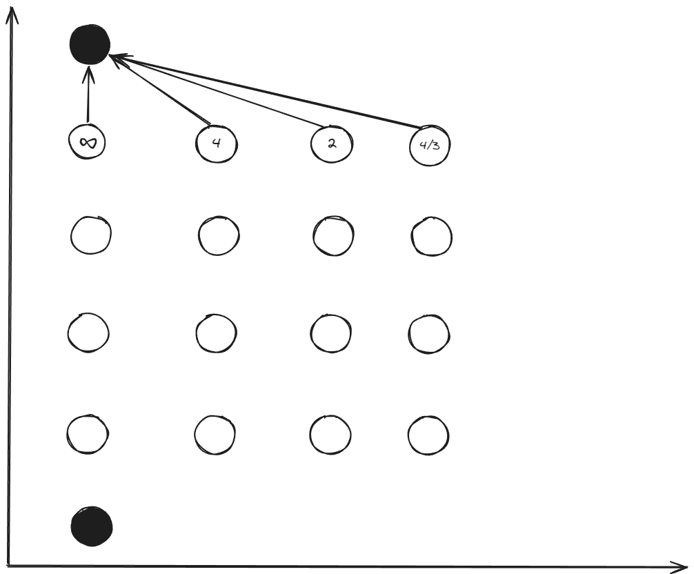

$4\to5$

$k=4: x_{[4_1]}=[6\;0]^T, x_{[4_2]}=[6\;1]^T, x_{[4_3]}=[6\;2]^T, x_{[4_4]}=[6\;3]^T$

For the $x_{[4_1]}$, there are 4 ways $4_1\to5_1,4_1\to5_2,4_1\to5_3,4_1\to5_4$ to select.

\[\Delta t_{[4_1\to5_1]}=\frac{2\Delta x_{1}}{x_{2[4_1]}+x_{2[5_1]}}=\frac{4}{0+0}=\infty\] \[u_{[4_1\to5_1]}=\frac{x_{2[5_1]}^{2}-x_{2[4_1]}^{2}}{2\Delta x_{1}}=\frac{0-0}{4}=0\] \[\Delta t_{[4_1\to5_2]}=\frac{2\Delta x_{1}}{x_{2[4_1]}+x_{2[5_2]}}=\frac{4}{1+0}=4\] \[u_{[4_1\to5_2]}=\frac{x_{2[5_2]}^{2}-x_{2[4_1]}^{2}}{2\Delta x_{1}}=\frac{1-0}{4}=\frac{1}{4}\] \[\Delta t_{[4_1\to5_3]}=\frac{2\Delta x_{1}}{x_{2[4_1]}+x_{2[5_3]}}=\frac{4}{0+2}=2\] \[u_{[4_1\to5_3]}=\frac{x_{2_{[5,3]}}^{2}-x_{2_{[4_1]}}^{2}}{2\Delta x_{1}}=\frac{4-0}{4}=1\] \[\Delta t_{[4_1\to5_4]}=\frac{2\Delta x_{1}}{x_{2_{[4_1]}}+x_{2_{[5_4]}}}=\frac{4}{3+0}=\frac{4}{3}\] \[u_{[4_1\to5_4]}=\frac{x_{2_{[5_4]}}^{2}-x_{2_{[4_1]}}^{2}}{2\Delta x_{1}}=\frac{9-0}{4}=\frac{9}{4}\]

The minimum time (cost) is $\Delta t_{ [4_1 \to 5_4] } = \frac{4}{3}$. However, the input $u_{ [4_1\to 5_4] }>2$ is not satisfied constraint condition. Therefor, the minimum cost to go for $x_{[4_1]}$ is

\[J^*_{[4_1\to5_3\to6]}=\Delta t_{4_1\to5_3}+J^*_{[5_3\to6]}=4\]

The optimal control is

\[u^*_{[4_1]}=u_{[4_1\to5_3]}=1\]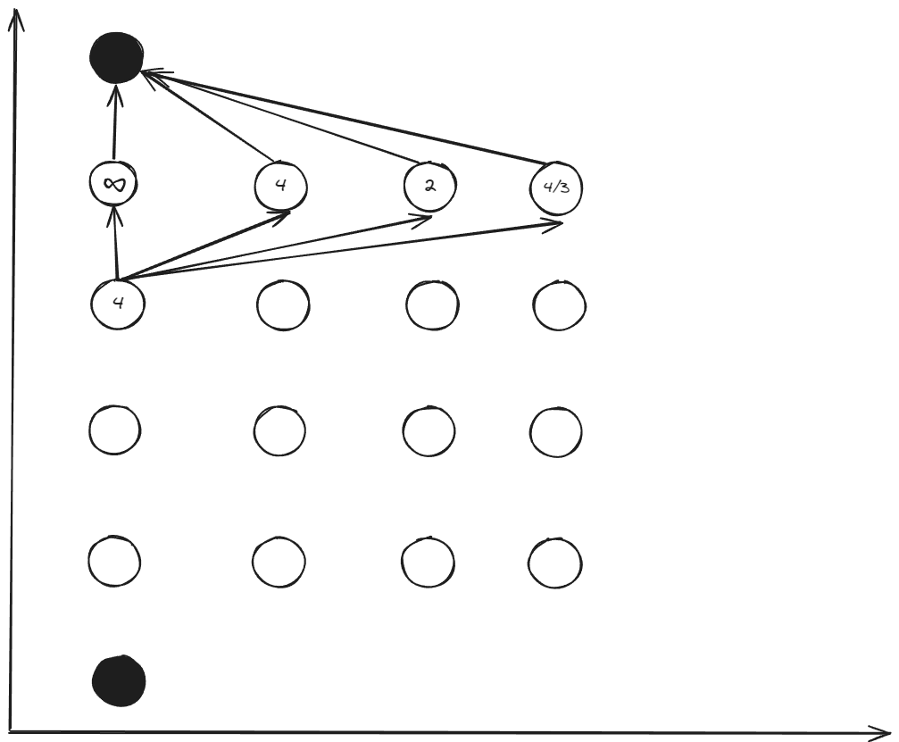

We calculated 4 paths for the $x_{[4_{1}]}$ , But only one optimal result $\Delta t_{[4_{1}\to5]}$ is retained to the node $x_{[4_{1}]}$ which be used by the state for $k<4$.

Same as above , consider the constraint condition, we can calculate the cost to go $J^*$ for the others node.

The table of cost to go:

Calculate times by backward multi stages:

\[(n_{x_1}-2)n_{x_2}^2+2\times x_2=72\]

Compared to the brute force method with exponential complexity, the backward multi stages has a linear relationship for $n_{x_1},n_{x_2}$. Therefore, it can improve computational efficiency and storage space.

Summary

The above calculation is the core algorithm of dynamic programming.
In the level $k$, it computes all selection for each node but retains only the optimal result $u^{*}_{k-node}$ by minimum cost to go $J^{*}_{[k\to k+1]}$. In the level $k-1$, only the cost to go from the level $k$ needs to be considered when computing the cost to go $J^{*}_{ [k-1\to k] }$. Because, whatever happened before, the optimal path from the current node to the end node has already been determined by the $J^{*}_{ [k\to k+1] }$ from the level $k$.

Additional, the above calculation can be off-line. Therefor, We can obtain the optimal control for each state, and just look at the table during the real-time control.

The table of optimal control input:

Code

  
clear
close all
set(0,'DefaultAxesFontName','Times New Roman')
set(0,'DefaultAxesFontSize',22)
rand('seed',1);
randn('seed',1);
%-------------------------------------------------------------------------------%
% DP %
% 12/14 by YANG GUANGZE %
% https://youkoutaku.github.io/ %
%-------------------------------------------------------------------------------%

%Initial state
h_init = 0;
v_init = 0;

%Final state
h_final =10;
v_final = 0;

%Boundary condition
h_min = 0;
h_max = 10;
N_h = 5; %Discretize for h
v_min = 0;
v_max = 3;
N_v = 3; %Discretize for v

%Create state array
Hd = h_min: (h_max - h_min)/N_h : h_max;
Vd = v_min: (v_max - v_min)/N_v : v_max;

%Input condition
u_min = -3;
u_max = 2;

% Define cost to go matrix
J_costtogo = zeros(N_h+1,N_v+1);

% Define input matrix
Input_acc = zeros(N_h+1,N_v+1);

%========== From 10m to 8m ==========%
v_avg = 0.5*( v_final + Vd); %average speed
T_delta = (h_max - h_min)./(N_h * v_avg); %time = cost
acc = (0 - Vd)./T_delta; %acceleration
J_temp = T_delta;
[acc_x, acc_y] = find( acc < u_min | acc > u_max); % Find which input is over the limit
Ind_lin_acc = sub2ind(size(acc), acc_x, acc_y); %Find linear index
J_temp(Ind_lin_acc) = inf; %put infitiy
J_costtogo(2,:) = J_temp;
Input_acc(2,:) = acc;
%========== From 8m to 2m ==========%
for k = 3:1:N_h
[Vd_x, Vd_y] = meshgrid(Vd, Vd);
v_avg = 0.5 * (Vd_x + Vd_y); %average speed
T_delta = (h_max - h_min)./(N_h * v_avg); %time = cost
acc = (Vd_y - Vd_x)./T_delta; %acceleration
J_temp = T_delta;
[acc_x, acc_y] = find( acc < u_min | acc > u_max); % Find which input is over the limit
Ind_lin_acc = sub2ind(size(acc), acc_x, acc_y); %Find linear index
J_temp(Ind_lin_acc) = inf; %put infitiy
J_temp = J_temp + meshgrid(J_costtogo(k-1,:))';
[J_costtogo(k,:), l]= min(J_temp); % l=acc
Ind_lin_acc = sub2ind(size(J_temp),l,1:length(l));
Input_acc(k,:) = acc(Ind_lin_acc);
end

%========== From 2m to 0m ==========%
v_avg = 0.5*( v_init + Vd); %average speed
T_delta = (h_max - h_min)./(N_h * v_avg); %time = cost
acc = (Vd - v_init)./T_delta; %acceleration
J_temp = T_delta;
[acc_x, acc_y] = find( acc < u_min | acc > u_max); % Find which input is over the limit
Ind_lin_acc = sub2ind(size(acc), acc_x, acc_y); %Find linear index
J_temp(Ind_lin_acc) = inf; %put infitiy
J_temp = J_temp + J_costtogo(5,:);
[J_costtogo(6,1), l]= min(J_temp); % l=acc
Ind_lin_acc = sub2ind(size(J_temp),l);
Input_acc(6,1) = acc(Ind_lin_acc);
%========== Plot ==========
h_plot_init = 0; % Initial height
v_plot_init = 0; % Initial velocity
acc_plot = zeros(length(Hd),1); % Define acc plot array
v_plot = zeros(length(Hd),1);% Define velocity plot array
h_plot = zeros(length(Hd),1);% Define height plot array
h_plot (1) = h_plot_init; % First value
v_plot (1) = v_plot_init; % First value

for k = 1 : 1 : N_h
[min_h,h_plot_index] = min(abs(h_plot(k) - Hd)); % Table look up
[min_v,v_plot_index] = min(abs(v_plot(k) - Vd)); % Table look up
acc_index = sub2ind(size(Input_acc), N_h+2-h_plot_index, v_plot_index); % Find control input /acceleration
acc_plot (k) = Input_acc(acc_index); % Save acceleration to the matrix
v_plot (k + 1) = sqrt((2 * (h_max - h_min)/N_h * acc_plot(k))+ v_plot (k)^2); % Calculate speed and height
h_plot (k + 1) = h_plot(k) + (h_max - h_min)/N_h;
end

%Plot
plot(v_plot,h_plot,'--^'),grid on;
xlabel('v(m)');
ylabel('h(m/s)');

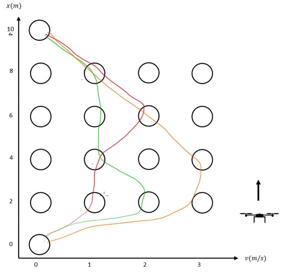
Simulation

Reference

Optimal Control by DR_CAN
王天威. 控制之美(卷2). 清华大学出版社. 2023.
Rakovic, S. V., & Levine, W. S. Handbook of model predictive control. 2018.
Dingyu Xue. Solving Optimization Problems with MATLAB. Tsinghua University Press, 2020.

Model Predict Control, Optimal Control

This post is licensed under CC BY 4.0 by the author.