中心極限定理(Central Limit Theorem)

Made by Youkoutaku

import numpy as np
from scipy import stats

import matplotlib.pyplot as plt
%matplotlib inline

%precision 3

np.random.seed(0)

(1) Reproductive property of normal distribution

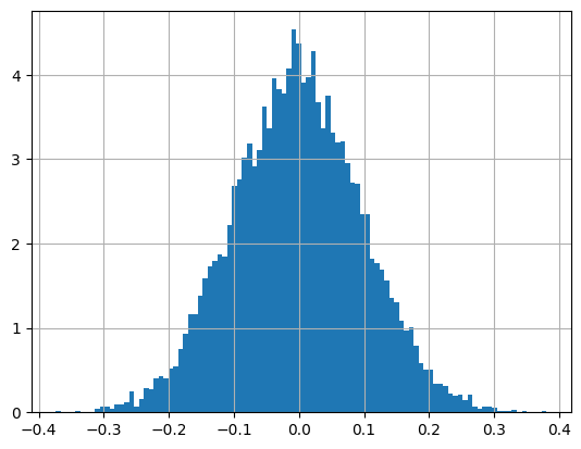
$X_1,X_2$がそれぞれ正規分布$N(m_1,σ_1^2)$と$N(m_1,σ_1^2)$に従う．

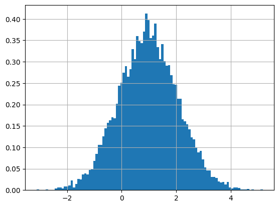
• $m_1=0, m_2=1$
• $σ_1=0.1, σ_2=0.5$
• $m=m_1+m_2, σ=σ_1+σ_2$

$X_1+X_2$は$N(m,σ^2)$に従うかどうかをシミュレーションで考察する．

#paramater
m1 = 0
m2 = 1
sigma1 = 0.1
sigma2 = 1

# X1
x1 = stats.norm.rvs(loc=m1, scale=sigma1, size=10000, random_state=0)
plt.hist(x1, density=True, bins=100)
plt.grid(True)
plt.show()

# X2
x2 = stats.norm.rvs(loc=m2, scale=sigma2, size=10000, random_state=0)
plt.hist(x2, density=True, bins=100)
plt.grid(True)
plt.show()

# X1+X2
plt.hist(x1+x2, density=True, bins=100)
plt.grid(True)
plt.show()

m = m1 + m2
sigma = sigma1 + sigma2

x = stats.norm.rvs(loc=m, scale=sigma, size=10000, random_state=0)
plt.hist(x, density=True, bins=100)
plt.grid(True)
plt.show()

よって，$X_1+X_2$ は $N(m,σ^2)$ に従うことを確認できた

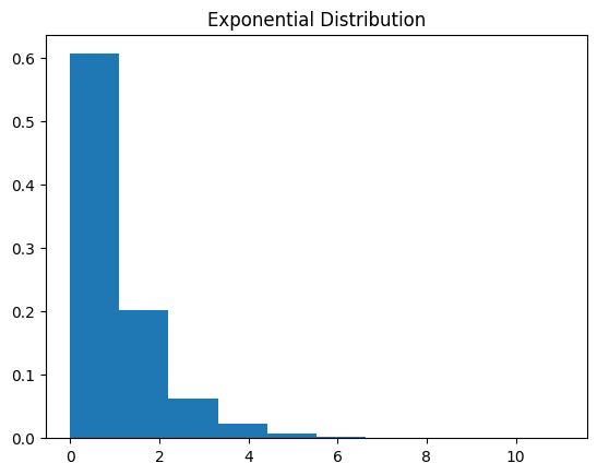
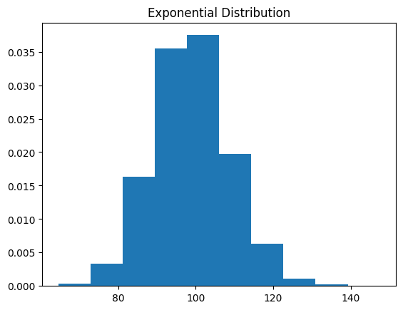
(2)Central limit theorem

指数分布と幾何分布により，中心極限定理の考察を行う．

#Exponential Distribution
def function_centrol_theory_expon(N):
  lambda_ = 1
  for i in range(N):
    new_data_expon = stats.expon.rvs(scale=1/lambda_, size=10000)
    if i<=1:
      data_expon = new_data_expon
    else:
      data_expon = data_expon + new_data_expon

  plt.hist(data_expon, density=True)
  plt.title('Exponential Distribution')
  plt.show()

# N=1, 10, 100
function_centrol_theory_expon(1)
function_centrol_theory_expon(10)
function_centrol_theory_expon(100)

#Geometric Distribution
def function_centrol_theory_geom(N):
  p = 0.5
  for i in range(N):
    rv_geom = stats.geom(p)
    new_data_geom = rv_geom.rvs(size=10000)
    if i<=1:
      data_geom = new_data_geom
    else:
      data_geom = data_geom + new_data_geom
  plt.hist(data_geom, density=True)
  plt.title('Geometric Distribution')
  plt.show()

# N=1, 10, 100
function_centrol_theory_geom(1)
function_centrol_theory_geom(10)
function_centrol_theory_geom(100)

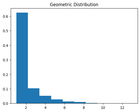
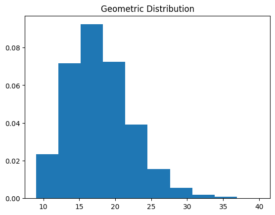
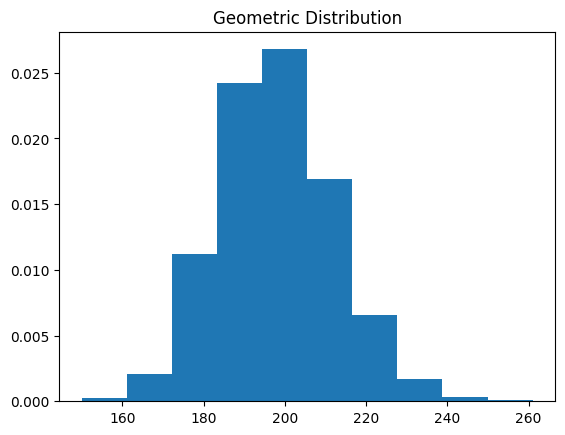
お互いに独立な確率変数の数 $N$ が高いほど，正規分布に近いことを確認し，中心極限定理をわかった．