Prescribed Performance Control (PPC)

Prescribed Performance Control (PPC) is a powerful control methodology that guarantees control system outputs/errors with desired transient performance as well as steady-state performance. This approach addresses one of the fundamental challenges in control systems: ensuring both excellent transient behavior and satisfactory steady-state characteristics.

Control Performance Importance

For control systems, transient performance is as important as steady-state performance. For some special dynamic systems, transient performance is even a higher priority index compared to the steady-state one. PPC has proven to be a powerful tool that addresses both aspects simultaneously.

Historical Background

The Prescribed Performance Control (PPC) methodology was first proposed by Bechlioulis in 2008 for the purpose of satisfying prescribed performance requirements in control systems. This groundbreaking approach revolutionized how engineers approach performance guarantees in control system design.

Core Components of PPC

The PPC methodology encompasses three fundamental issues:

1. Performance Function

• Applied to impose boundary constraints on tracking errors
• Defines the allowable error evolution over time
• Provides mathematical framework for performance specification

2. Equivalent Transformation

• Based on the error transformation approach
• Defines a transformed error that is easier to work with
• Enables "unconstrained" controller design for constrained problems

3. Controller Design

• Uses the transformed error instead of the original tracking error
• Applies standard control techniques to the transformed system
• Guarantees original performance specifications

Performance Function Theory

Mathematical Definition

The performance function $P(t)$ must satisfy the following properties:

• $P(t)$ is smooth, positive, and decreasing for all $t \geq 0$
• $\lim_{t \to 0} P(t) = p_0$ and $\lim_{t \to \infty} P(t) = p_{\infty}$
• $p_0 > p_{\infty} > 0$

Standard Performance Function: $P(t) = (p_0 - p_{\infty})e^{-e^{\iota t}} + p_{\infty}$

where $p_0, p_{\infty}, \iota \in \mathbb{R}^{+}$.

Performance Function Properties

• Bounded Range: $P(t) \in [p_{\infty}, p_0)$
• Convergence Rate: $\iota$ controls the convergence rate of $P(t)$
• Initial Performance: $p_0$ sets the initial error bound
• Steady-State Performance: $p_{\infty}$ defines the ultimate error bound

Error Constraints

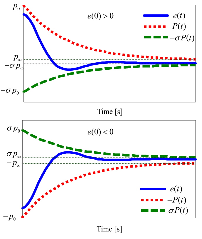
The tracking error $e(t)$ must satisfy:

$$\begin{cases} -\sigma P(t) < e(t) < P(t), & \text{if } e(0) > 0 \\ -P(t) < e(t) < \sigma P(t), & \text{if } e(0) < 0 \end{cases}$$

where $0 \leq \sigma \leq 1$ for all $t \geq 0$.

Performance Guarantee

By appropriately choosing $p_0$, $p_{\infty}$, and $\iota$ for $P(t)$, the transient performance such as overshoot and convergence time of $e(t)$ can be guaranteed. Moreover, steady-state performance can also be achieved:

• $-\sigma p_{\infty} < e(\infty) < p_{\infty}$ (for $e(0) > 0$)
• $-p_{\infty} < e(\infty) < \sigma p_{\infty}$ (for $e(0) < 0$)

Error Transformation

Motivation

Direct controller development using the constrained system is impossible. The error transformation approach transforms the constrained problem into an "unconstrained" formulation that is amenable to standard control design techniques.

Transformation Relationship

$$e(t) = E(\xi)P(t)$$

where:

• $\xi$ is the transformed error
• $E(\xi)$ is the transformation function

Transformation Function Properties

The function $E(\xi)$ must satisfy:

1. Smoothness: $E(\xi)$ is smooth, bounded, and strictly increasing
2. Range Constraints:
   • $E(\xi) \in (-\sigma, 1)$ if $e(0) > 0$
   • $E(\xi) \in (-1, \sigma)$ if $e(0) < 0$
3. Limit Behavior:
   • If $e(0) > 0$: $\lim_{\xi \to -\infty} E(\xi) = -\sigma$ and $\lim_{\xi \to +\infty} E(\xi) = 1$
   • If $e(0) < 0$: $\lim_{\xi \to -\infty} E(\xi) = -1$ and $\lim_{\xi \to +\infty} E(\xi) = \sigma$

Explicit Transformation Function

$$E(\xi) = \begin{cases} \frac{e^{\xi} - \sigma e^{-\xi}}{e^{\xi} + e^{-\xi}}, & \text{if } e(0) \geq 0 \\ \frac{\sigma e^{\xi} - e^{-\xi}}{e^{\xi} + e^{-\xi}}, & \text{if } e(0) < 0 \end{cases}$$

Inverse Transformation

The transformed error is obtained as:

$$\begin{aligned}\xi = E^{-1}\left(\frac{e(t)}{P(t)}\right) = \begin{cases}\frac{1}{2}\ln\left(\frac{e(t)/P(t) + \sigma}{1 - e(t)/P(t)}\right), & \text{if } e(0) \geq 0 \\\frac{1}{2}\ln\left(\frac{e(t)/P(t) + 1}{\sigma - e(t)/P(t)}\right), & \text{if } e(0) < 0\end{cases}\end{aligned}$$

where $E^{-1}$ is the inverse function.

Controller Design Based on PPC

System Model

Consider a Single-Input Single-Output (SISO) dynamic system:

$$\dot x = f(x) + g(x)u$$

where:

• $x$ is the system state
• $u$ is the control input
• $f(x), g(x)$ are continuous functions

Tracking Error Definition

$$\begin{aligned}e(t) = x - x ^ { \text { ref } }\end{aligned}$$

Transformed Error Dynamics

The dynamics of the transformed error are given by:

$$\begin{aligned} \dot \xi = \Delta _ { \xi } \left(\dot{e}(t) - \frac{\dot{P}(t)}{P(t)}e(t)\right) \end{aligned}$$ $$\begin{aligned}= \Delta_{\xi}\left(f(x) + g(x)u - \dot x ^{\text{ref}} - \frac{\dot{P}(t)}{P(t)}e(t)\right)\end{aligned}$$

where the transformation gain $\Delta_{\xi}$ is:

$$\begin{aligned}\Delta_{\xi} = \begin{cases}\frac{1 + \sigma}{2P(t)[e(t)/P(t) + \sigma][1 - e(t)/P(t)]} > 0, & \text{if } e(0) \geq 0 \\\frac{1 + \sigma}{2P(t)[e(t)/P(t) + 1][\sigma - e(t)/P(t)]} > 0, & \text{if } e(0) < 0\end{cases}\end{aligned}$$

Lyapunov-Based Controller Design

Using the transformed error $\xi$, controller design becomes straightforward using Lyapunov synthesis:

Lyapunov Function:

$$V(\xi) = \frac{1}{2}\xi^T\xi$$

Lyapunov Derivative:

$$\begin{aligned}\dot { V } (\xi) = \xi^T \dot{\xi}\end{aligned}$$

Stability Condition: Design the input $u$ to satisfy:

$$\dot V (\xi) + V(\xi) \leq 0$$

This ensures exponential convergence of $\xi$ to zero, which guarantees that the original error $e(t)$ remains within the prescribed performance bounds.

Simplified Formulation

Asymmetric Constraints

If the initial value of tracking error $e(t)$ is known, the constraint boundary can be simplified using asymmetric bounds:

$$-\sigma_L P(t) < e(t) < \sigma_R P(t)$$

Generalized Transformation Function

$$\begin{aligned}E(\xi) = \frac{\sigma_R e^{\xi} - \sigma_L e^{-\xi}}{e^{\xi} + e^{-\xi}}\end{aligned}$$

Simplified Inverse Transformation

$$\begin{aligned}\xi = E^{-1}\left(\frac{e(t)}{P(t)}\right) = \frac{1}{2}\ln\left(\frac{e(t)/P(t) + \sigma_L}{\sigma_R - e(t)/P(t)}\right)\end{aligned}$$

Simplified Transformation Gain

$$\begin{aligned}\Delta _ { \xi } = \frac{1}{2P(t)(e(t)/P(t) + \sigma_L)} - \frac{1}{2P(t)(e(t)/P(t) - \sigma_R)} > 0\end{aligned}$$

Advantages of PPC

1. Performance Guarantees

• Mathematically rigorous bounds on transient behavior
• Guaranteed steady-state performance
• Predictable system response

2. Design Flexibility

• Adjustable performance parameters ($p_0$, $p_{\infty}$, $\iota$)
• Customizable constraint boundaries
• Adaptable to various system requirements

3. Theoretical Rigor

• Lyapunov stability guarantees
• Well-established mathematical foundation
• Proven convergence properties

4. Practical Implementation

• Systematic design procedure
• Compatible with existing control techniques
• Applicable to various system classes

Applications and Extensions

Application Areas

• Robotic Systems: Precise trajectory tracking with performance bounds
• Aerospace Control: Attitude control with guaranteed transient response
• Process Control: Chemical processes with strict performance requirements
• Automotive Control: Vehicle dynamics with safety constraints

Recent Extensions

• Adaptive PPC: For systems with unknown parameters
• Robust PPC: For systems with uncertainties and disturbances
• Multi-Agent PPC: For distributed control systems
• Output Feedback PPC: For systems with limited state information

Summary

Prescribed Performance Control represents a significant advancement in control theory, providing:

1. Unified Framework: Addresses both transient and steady-state performance
2. Mathematical Rigor: Well-established theoretical foundation
3. Practical Utility: Systematic design approach for real-world systems
4. Performance Guarantees: Mathematically proven performance bounds

The PPC methodology transforms the challenging problem of constrained performance into a manageable unconstrained control design problem, making it an invaluable tool for modern control engineers.

References

1. Prescribed performance control approaches, applications and challenges: A comprehensive survey - Bu (2023) - Asian Journal of Control - Wiley Online Library
2. Robust Adaptive Control of Feedback Linearizable MIMO Nonlinear Systems With Prescribed Performance - IEEE Transactions on Automatic Control
3. Prescribed performance adaptive control of SISO feedback linearizable systems with disturbances - IEEE Conference Publication

Further Reading

For advanced topics and recent developments in PPC, refer to the latest research publications and survey papers that cover adaptive, robust, and distributed extensions of the basic PPC framework.