Optimal Control Problem Formulation

This document introduces the fundamental concepts of optimal control problems using the unicycle model as a practical example. We explore different control objectives from basic parking problems to advanced collision avoidance scenarios.

Unicycle Model

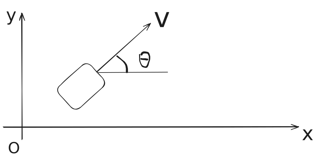
The unicycle model serves as an excellent example for understanding nonlinear optimal control problems due to its simplicity and practical relevance in robotics.

State Space Representation

The state vector is defined as:

$$x(t) = \begin{bmatrix} x_1(t) \\ x_2(t) \\ x_3(t) \\ x_4(t) \end{bmatrix} = \begin{bmatrix} p_x(t) \\ p_y(t) \\ v(t) \\ \theta(t) \end{bmatrix}$$

Where:

• $p_x(t)$: position in x direction
• $p_y(t)$: position in y direction
• $v(t)$: linear velocity
• $\theta(t)$: wheel orientation angle

Control Input

The control input vector is:

$$u(t) = \begin{bmatrix} u_1(t) \\ u_2(t) \end{bmatrix} = \begin{bmatrix} \alpha(t) \\ \omega(t) \end{bmatrix}$$

Where:

• $\alpha(t)$: linear acceleration
• $\omega(t)$: angular velocity

Continuous-Time Dynamics

The state equation for the unicycle model is:

$$\dot{x}(t) = \begin{bmatrix} v(t)\cos{\theta(t)} \\ v(t)\sin{\theta(t)} \\ 0 \\ 0 \end{bmatrix} + \begin{bmatrix} 0 \\ 0 \\ \alpha(t) \\ \omega(t) \end{bmatrix} = f(x(t), u(t))$$

Nonlinearity

This is a nonlinear system due to the trigonometric functions in the kinematic equations.

Discretization

For numerical implementation, we discretize the system with sample time $T_s$: $x[k+1] = f_d(x[k], u[k])$

where $f_d$ represents the discrete-time dynamics obtained through numerical integration methods.

Problem 1: Parking Problem

The parking problem represents the most basic optimal control scenario - moving from an initial state to a desired final state.

Problem Setup

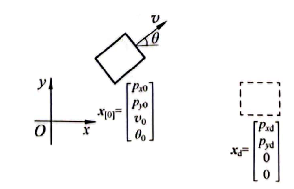
System: Discrete-time unicycle model $x[k+1] = f_d(x[k], u[k])$

Initial and target states:

$$x[0] = \begin{bmatrix} p_{x0} \\ p_{y0} \\ v_0 \\ \theta_0 \end{bmatrix}, \quad x_d = \begin{bmatrix} p_{xd} \\ p_{yd} \\ 0 \\ 0 \end{bmatrix}$$

Terminal state: At time $k = N$: $x[N] = f_d[\cdots[f_d[x[0], u[0]], u[1], \ldots, u[N-1]]]$

Key Insight

The final state depends only on the initial state and the sequence of control inputs $u[0], u[1], \ldots, u[N-1]$.

Performance Function

The basic performance function (cost function) is:

$$\begin{aligned} J &= (x_1[N] - x_{d1})^2 + (x_2[N] - x_{d2})^2 + (x_3[N] - x_{d3})^2 + (x_4[N] - x_{d4})^2 \\ &= (x[N] - x_d)^T(x[N] - x_d) = \|x[N] - x_d\|^2 \\ &= e[N]^T e[N] = \|e[N]\|^2 \end{aligned}$$

where $e[k] = x[k] - x_d$ is the error vector.

Control Policy

The optimal control policy seeks: $u^* = [u[0], u[1], \ldots, u[N-1]] = \arg\min_{u \in \Omega} J$

where $\Omega$ is the set of admissible controls.

Weight Matrix

To prioritize certain states, we introduce a weight matrix: $J = e[N]^T S e[N] \triangleq \|x[N] - x_d\|_S^2$

where $S$ is a positive semi-definite symmetric matrix ($x^T S x \geq 0$ and $s_{ij} = s_{ji}$).

Weight Matrix Properties

• Usually diagonal: $s_{ij} = 0$ for $i \neq j$
• Larger diagonal elements indicate higher importance of corresponding states
• Must be positive semi-definite for convexity

Constraints

Physical limitations impose constraints:

State constraints: $-v_{\max} < v[k] < v_{\max}$

Input constraints: $u_{\min} < u[k] < u_{\max}$

Hard Constraints

These are hard constraints that must be strictly satisfied during system operation.

Problem 2: Input Cost Consideration

Real systems require energy to operate, making input cost an important consideration.

Soft Constraints

Unlike hard constraints, soft constraints aren't strictly enforced but are penalized in the cost function.

Modified Cost Function

$J = \|x[N] - x_d\|_S^2 + \sum_{k=0}^{N-1} \|u[k]\|_R^2$

Where:

• $\|x[N] - x_d\|_S^2 = (x[N] - x_d)^T S (x[N] - x_d)$: terminal cost
• $\|u[k]\|_R^2 = u[k]^T R u[k]$: input cost
• $S$: reference weight matrix
• $R$: input cost weight matrix

Design Trade-offs

The relative weighting determines system behavior:

$S \gg R$: Control performance is more important!

$R \gg S$: Input cost is more important!

Problem 3: Trajectory Tracking

Moving beyond point-to-point control, trajectory tracking follows a time-varying reference.

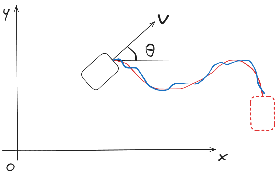
Reference Trajectory

$x_d[k] = \begin{bmatrix} p_{xd}[k] \\ p_{yd}[k] \\ 0 \\ 0 \end{bmatrix}$

Performance Function

$J = \|x[N] - x_d[N]\|_S^2 + \sum_{k=0}^{N-1} \left(\|x[k] - x_d[k]\|_Q^2 + \|u[k]\|_R^2\right)$

where $Q$ is the trajectory weight matrix that penalizes deviations from the reference path at each time step.

Problem 4: Collision Avoidance

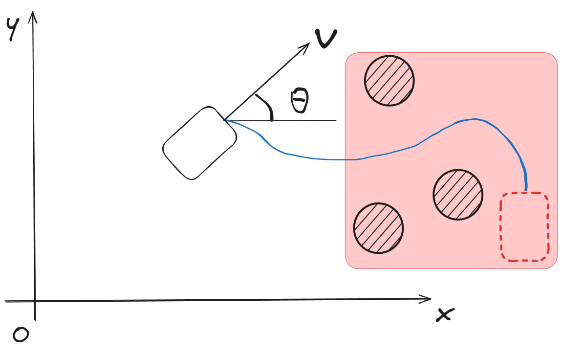
Advanced control problems must consider safety and obstacle avoidance.

Method 1: Hard Constraint Approach

Add constraint conditions to Problem 3: $(p_x[k], p_y[k]) \notin (p_{xo}, p_{yo})$

where $(p_{xo}, p_{yo}) \in \Omega_o$ represents the obstacle space.

Method 2: Soft Constraint Approach

Modify the cost function to penalize proximity to obstacles:

$J = \|x[N] - x_d[N]\|_S^2 + \sum_{k=0}^{N-1} \left(\|x[k] - x_d[k]\|_Q^2 + \|u[k]\|_R^2\right) + \sum_{k=0}^{N-1} D^{-1}[k]_P$

Where:

• $D[k]$: distance from object to obstacle at time $k$
• $P$: weight matrix for distance penalty
• $D^{-1}[k]_P$: penalty that increases as distance decreases

General Optimal Control Problem Formulation

System Model

$x[k+1] = f_d(x[k], u[k], k)$

Reference

$x_d[k] \text{ (may be time-varying)}$

Performance Function

$J = h(x[N], x_d[N], N) + \sum_{k=0}^{N-1} g(x[k], x_d[k], u[k], k)$

Constraints

• State constraints: $x[k] \in X$ (admissible trajectory set)
• Input constraints: $u[k] \in \Omega$ (admissible control set)

Feasibility

There must be at least one feasible solution within the constraints. Overly restrictive constraints can lead to infeasible problems.

Common Optimal Control Problem Types

1. Minimum Time Problem

$J = \sum_{k=0}^N 1 = N$

Objective: Reach the target in minimum time.

2. Terminal Control Problem

$J = \|x[N] - x_d[N]\|_S^2$

Objective: Minimize final state error.

3. Minimum Input Problem

$J = \sum_{k=0}^N \|u[k]\|_{R[k]}^2$

Objective: Minimize control effort.

4. Trajectory Tracking Problem

$J = \sum_{k=0}^N \|x[k] - x_d[k]\|_{Q[k]}^2$

Objective: Follow reference trajectory closely.

5. General Optimal Control Problem

$J = \|x[N] - x_d[N]\|_S^2 + \sum_{k=0}^{N-1} \left(\|x[k] - x_d[k]\|_{Q[k]}^2 + \|u[k]\|_{R[k]}^2\right)$

Objective: Balance terminal accuracy, trajectory tracking, and input cost.

6. Regulator Problem

When $x_d[k] = 0$, the problem becomes a regulator problem: $J = \|x[N]\|_S^2 + \sum_{k=0}^{N-1} \left(\|x[k]\|_{Q[k]}^2 + \|u[k]\|_{R[k]}^2\right)$

Problem Transformation

For trajectory problems, introduce error $e[k] = x[k] - x_d[k]$ and formulate the error dynamics. The control task becomes driving $e[k] \to 0$, which can be solved as a regulator problem.

Solution Approaches

Different optimal control problems require different solution methods:

1. Linear Quadratic Regulator (LQR): For linear systems with quadratic costs
2. Dynamic Programming: For general nonlinear problems
3. Model Predictive Control (MPC): For real-time implementation with constraints
4. Pontryagin's Maximum Principle: For continuous-time problems
5. Direct Methods: Numerical optimization of discretized problems

References

1. Optimal Control by DR_CAN
2. Wang, T. (2023). 控制之美 (卷2). Tsinghua University Press.
3. Grüne, L., & Pannek, J. (2017). Nonlinear Model Predictive Control. Springer.
4. Kirk, D. E. (2004). Optimal Control Theory: An Introduction. Dover Publications.