LQR for Time-Varying Reference Tracking

Linear Quadratic Regulator (LQR) for tracking time-varying reference signals extends the set-point regulation framework to handle dynamic references. This approach uses incremental input optimization to achieve smooth tracking performance.

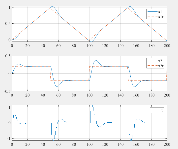
Problem Overview

Set-Point vs. Tracking Control

Set-Point Regulation: Track constant reference values $x^r_k = \text{constant}$

Tracking Control: Follow time-varying reference trajectories
$x^r_k = f(k) \text{ (time-varying)}$

The tracking problem is more challenging because:

• Reference changes require responsive control
• Smooth control action is desired to avoid actuator stress
• Trade-off between tracking performance and control effort

Problem Formulation

System Dynamics

Consider a discrete-time linear system: $x_{k+1} = f(x_k, u_k) = Ax_k + Bu_k$

Where:

• $x_k \in \mathbb{R}^n$: system state
• $u_k \in \mathbb{R}^p$: control input
• $A \in \mathbb{R}^{n \times n}$: state transition matrix
• $B \in \mathbb{R}^{n \times p}$: input matrix

Reference Dynamics

The time-varying reference signal evolves as: $x^r_{k+1} = A_r x^r_k$

Where $A_r$ describes the reference dynamics (may include integrators, oscillators, etc.).

Key Innovation: Incremental Input

Instead of optimizing the control input $u_k$ directly, we optimize the incremental input: $\Delta u_k = u_k - u_{k-1}$

This leads to: $u_k = \Delta u_k + u_{k-1}$

Why Incremental Input?

• Smoother control: Penalizes rapid changes in control action
• Better tracking: Reduces control chattering
• Actuator friendly: Limits slew rate naturally
• Improved robustness: More conservative control behavior

Modified System Dynamics

Substituting the incremental input: $x_{k+1} = Ax_k + B(\Delta u_k + u_{k-1}) = Ax_k + Bu_{k-1} + B\Delta u_k$

State Augmentation

Augmented State Vector

To handle both reference tracking and incremental input, we augment the state: $z_k := \begin{bmatrix} x_k \\ x^r_k \\ u_{k-1} \end{bmatrix}$

Augmented System Dynamics

The augmented system becomes: $z_{k+1} = A_z z_k + B_z \Delta u_k$

Where: $A_z := \begin{bmatrix} A & 0_{n \times n} & B \\ 0_{n \times n} & A_r & 0_{n \times p} \\ 0_{p \times n} & 0_{p \times n} & I_{p \times p} \end{bmatrix}$

$B_z := \begin{bmatrix} B \\ 0_{n \times p} \\ I_{p \times p} \end{bmatrix}$

Tracking Error

The tracking error is extracted from the augmented state: $e_k = x_k - x^r_k = [I_{n \times n} \quad -I_{n \times n} \quad 0_{n \times p}] z_k = C_z z_k$

Where $C_z = [I_{n \times n} \quad -I_{n \times n} \quad 0_{n \times p}]$ is the error extraction matrix.

Cost Function Formulation

Quadratic Performance Function

The objective is to minimize: $J = h(e_N) + \sum_{k=0}^{N-1} g(e_k, \Delta u_k)$

Where: $h(e_N) = \frac{1}{2} e_N^T S e_N$ $g(e_k, \Delta u_k) = \frac{1}{2} [e_k^T Q e_k + \Delta u_k^T R \Delta u_k]$

Key Difference

Note that we penalize the incremental input $\Delta u_k$, not the absolute input $u_k$. This promotes smooth control action.

Transformation to Augmented Variables

Substituting the error definition: $J = \frac{1}{2} (C_z z_N)^T S (C_z z_N) + \frac{1}{2} \sum_{k=0}^{N-1} [(C_z z_k)^T Q C_z z_k + \Delta u_k^T R \Delta u_k]$

Simplifying: $J = \frac{1}{2} z_N^T S^z z_N + \frac{1}{2} \sum_{k=0}^{N-1} [z_k^T Q^z z_k + \Delta u_k^T R \Delta u_k]$

Where: $S^z = C_z^T S C_z$ $Q^z = C_z^T Q C_z$

LQR Solution

Optimal Incremental Input

The optimal incremental input is: $\Delta u^*_{N-k} = -F_{N-k} z_{N-k}$

Feedback Gain

The optimal feedback gain is: $F_{N-k} = (B_z^T P_{k-1} B_z + R)^{-1} B_z^T P_{k-1} A_z$

Cost-to-Go Matrix

The cost-to-go matrix evolves according to: $P_k = (A_z - B_z F_{N-k})^T P_{k-1} (A_z - B_z F_{N-k}) + F_{N-k}^T R F_{N-k} + Q^z$

With terminal condition: $P_0 = S^z$

Control Implementation

The actual control input is computed as: $u^*_k = \Delta u^*_k + u^*_{k-1}$

Example: Double Integrator Tracking

System Setup

Consider a second-order system (double integrator): $\begin{bmatrix} \dot{x}_1 \\ \dot{x}_2 \end{bmatrix} = \begin{bmatrix} 0 & 1 \\ 0 & 0 \end{bmatrix} \begin{bmatrix} x_1 \\ x_2 \end{bmatrix} + \begin{bmatrix} 0 \\ 1 \end{bmatrix} u(t)$

Initial reference: $x^r(0) = \begin{bmatrix} 0 \\ 0.2 \end{bmatrix}$

Step changes in velocity reference:

• At $k = 50$: $x^r_2 = -0.2$
• At $k = 100$: $x^r_2 = 0.2$
• At $k = 150$: $x^r_2 = -0.2$
• At $k = 200$: $x^r_2 = 0.2$

Weight Matrices

$Q = \begin{bmatrix} 1 & 0 \\ 0 & 1 \end{bmatrix}, \quad S = \begin{bmatrix} 1 & 0 \\ 0 & 1 \end{bmatrix}, \quad R = 0.1$

MATLAB Implementation

%% LQR for Time-Varying Reference Tracking
%-----------------------------------------------%
% Youkoutaku: https://youkoutaku.github.io/
% Date: 2024/10/07
% Description: LQR for tracking time-varying reference signals
%-----------------------------------------------%
clear; close all; clc;
set(0, 'DefaultAxesFontName', 'Times New Roman')
set(0, 'DefaultAxesFontSize', 14)

%% System Model
A = [0 1; 0 0];
n = size(A, 1);
B = [0; 1];
p = size(B, 2);
C = [1 0; 0 1];
D = [0; 0];

%% System Discretization
Ts = 0.1; % Sample time
sys_d = c2d(ss(A, B, C, D), Ts);
A = sys_d.a; % Discretized system matrix A
B = sys_d.b; % Discretized input matrix B

%% Weight Matrices
Q = [1 0; 0 1]; % Tracking error weight
S = [1 0; 0 1]; % Terminal weight
R = 0.1;        % Incremental input weight

%% Initial Conditions
x0 = [0; 0];
x = x0;
u0 = 0;
u = u0;

%% Reference Signal Setup
xr = [0; 0.2];
% Reference dynamics (constant velocity in this case)
Ar = c2d(ss([0 1; 0 0], [0; 0], [1 0; 0 1], [0; 0]), Ts).A;

% Initial augmented state
z = [x; xr; u];

%% Augmented System Construction
[Az, Bz, Qz, Rz, Sz] = Augmented_System_Input(A, B, Q, R, S, Ar);

%% LQR Gain Computation
[F] = LQR_DP(Az, Bz, Qz, Rz, Sz);

%% Simulation
k_steps = 200;
x_h = zeros(n, k_steps + 1);
x_h(:, 1) = x;
u_h = zeros(p, k_steps + 1);
u_h(:, 1) = u;
xr_h = zeros(n, k_steps + 1);
xr_h(:, 1) = xr;
Delta_u_h = zeros(p, k_steps);

for k = 1:k_steps
    % Time-varying reference signal
    if k == 50
        xr = [xr(1); -0.2];
    elseif k == 100
        xr = [xr(1); 0.2];
    elseif k == 150
        xr = [xr(1); -0.2];
    elseif k == 200
        xr = [xr(1); 0.2];
    end
    
    % Compute incremental input
    Delta_u = -F * z;
    Delta_u_h(:, k) = Delta_u;
    
    % Compute total input
    u = Delta_u + u;
    
    % Update system
    x = A * x + B * u;
    xr = Ar * xr;
    z = [x; xr; u];
    
    % Store results
    x_h(:, k + 1) = x;
    u_h(:, k + 1) = u;
    xr_h(:, k + 1) = xr;
end

%% Plotting Results
figure('Position', [100, 100, 800, 600]);

% Position tracking
subplot(3, 1, 1);
plot(0:k_steps, x_h(1, :), 'b-', 'LineWidth', 2);
hold on;
plot(0:k_steps, xr_h(1, :), 'r--', 'LineWidth', 2);
legend('x_1', 'x_1^r', 'FontSize', 12);
xlabel('Time step');
ylabel('Position');
title('Position Tracking');
xlim([0 k_steps]);
grid on;

% Velocity tracking
subplot(3, 1, 2);
plot(0:k_steps, x_h(2, :), 'b-', 'LineWidth', 2);
hold on;
plot(0:k_steps, xr_h(2, :), 'r--', 'LineWidth', 2);
legend('x_2', 'x_2^r', 'FontSize', 12);
xlabel('Time step');
ylabel('Velocity');
title('Velocity Tracking');
xlim([0 k_steps]);
grid on;

% Control input
subplot(3, 1, 3);
stairs(0:k_steps, u_h(1, :), 'b-', 'LineWidth', 2);
legend('u', 'FontSize', 12);
xlabel('Time step');
ylabel('Control Input');
title('Control Effort');
xlim([0 k_steps]);
grid on;

sgtitle('LQR Time-Varying Reference Tracking', 'FontSize', 16, 'FontWeight', 'bold');

%% Helper Functions
function [Az, Bz, Qz, Rz, Sz] = Augmented_System_Input(A, B, Q, R, S, Ar)
    % Create augmented system for incremental input optimization
    n = size(A, 1);
    p = size(B, 2);
    
    % Augmented system matrices
    Az = [A, zeros(n), B;
          zeros(n), Ar, zeros(n, p);
          zeros(p, n), zeros(p, n), eye(p)];
    
    Bz = [B; zeros(n, p); eye(p)];
    
    % Error extraction matrix
    Cz = [eye(n), -eye(n), zeros(n, p)];
    
    % Augmented weight matrices
    Sz = Cz' * S * Cz;
    Qz = Cz' * Q * Cz;
    Rz = R;
end

function [F] = LQR_DP(A, B, Q, R, S)
    % LQR solution using dynamic programming
    P0 = S;
    max_iter = 200;
    tolerance = 1e-6;
    
    P_k_minus_1 = P0;
    F_prev = inf;
    
    for k = 1:max_iter
        F_current = (R + B' * P_k_minus_1 * B) \ (B' * P_k_minus_1 * A);
        P_k = (A - B * F_current)' * P_k_minus_1 * (A - B * F_current) + ...
              F_current' * R * F_current + Q;
        
        if max(abs(F_current - F_prev), [], 'all') < tolerance
            fprintf('LQR converged in %d iterations\n', k);
            F = F_current;
            return;
        end
        
        P_k_minus_1 = P_k;
        F_prev = F_current;
    end
    
    error('LQR did not converge');
end

Python Implementation

import numpy as np
import matplotlib.pyplot as plt
from scipy.linalg import solve_discrete_are

def augmented_system_input(A, B, Q, R, S, Ar):
    """Create augmented system for incremental input optimization"""
    n = A.shape[0]
    p = B.shape[1]
    
    # Augmented system matrices
    Az = np.block([[A, np.zeros((n, n)), B],
                   [np.zeros((n, n)), Ar, np.zeros((n, p))],
                   [np.zeros((p, n)), np.zeros((p, n)), np.eye(p)]])
    
    Bz = np.block([[B],
                   [np.zeros((n, p))],
                   [np.eye(p)]])
    
    # Error extraction matrix
    Cz = np.block([np.eye(n), -np.eye(n), np.zeros((n, p))])
    
    # Augmented weight matrices
    Sz = Cz.T @ S @ Cz
    Qz = Cz.T @ Q @ Cz
    Rz = R
    
    return Az, Bz, Qz, Rz, Sz

def lqr_tracking(A, B, Q, R, S, Ar, x0, u0, reference_profile, k_steps):
    """
    LQR for time-varying reference tracking
    """
    n = A.shape[0]
    p = B.shape[1]
    
    # Create augmented system
    Az, Bz, Qz, Rz, Sz = augmented_system_input(A, B, Q, R, S, Ar)
    
    # Solve Riccati equation
    P = solve_discrete_are(Az, Bz, Qz, Rz, s=Sz)
    F = np.linalg.solve(Rz + Bz.T @ P @ Bz, Bz.T @ P @ Az)
    
    # Initialize simulation
    x_traj = np.zeros((n, k_steps + 1))
    u_traj = np.zeros((p, k_steps + 1))
    xr_traj = np.zeros((n, k_steps + 1))
    delta_u_traj = np.zeros((p, k_steps))
    
    x_traj[:, 0] = x0
    u_traj[:, 0] = u0
    xr_traj[:, 0] = reference_profile(0)
    
    x = x0.copy()
    u = u0
    xr = reference_profile(0)
    
    # Simulation loop
    for k in range(k_steps):
        # Update reference
        xr = reference_profile(k + 1)
        
        # Augmented state
        z = np.concatenate([x, xr, u])
        
        # Compute incremental input
        delta_u = -F @ z
        delta_u_traj[:, k] = delta_u
        
        # Compute total input
        u = delta_u + u
        
        # Update system
        x = A @ x + B @ u
        xr = Ar @ xr
        
        # Store results
        x_traj[:, k + 1] = x
        u_traj[:, k + 1] = u
        xr_traj[:, k + 1] = xr
    
    return x_traj, u_traj, xr_traj, delta_u_traj

# System matrices
A = np.array([[0, 1], [0, 0]])
B = np.array([[0], [1]])

# Discretize system
from scipy.signal import cont2discrete
Ts = 0.1
A_d, B_d, _, _, _ = cont2discrete((A, B, np.eye(2), np.zeros((2, 1))), Ts)

# Reference dynamics (constant velocity)
Ar = np.array([[1, Ts], [0, 1]])

# Weight matrices
Q = np.eye(2)
S = np.eye(2)
R = np.array([[0.1]])

# Initial conditions
x0 = np.array([0, 0])
u0 = np.array([0])

# Define reference profile
def reference_profile(k):
    """Step changes in velocity reference"""
    if k < 50:
        return np.array([0, 0.2])
    elif k < 100:
        return np.array([0, -0.2])
    elif k < 150:
        return np.array([0, 0.2])
    elif k < 200:
        return np.array([0, -0.2])
    else:
        return np.array([0, 0.2])

# Simulate
k_steps = 200
x_traj, u_traj, xr_traj, delta_u_traj = lqr_tracking(
    A_d, B_d, Q, R, S, Ar, x0, u0, reference_profile, k_steps)

# Plotting
fig, (ax1, ax2, ax3) = plt.subplots(3, 1, figsize=(10, 8))
time_steps = np.arange(k_steps + 1)

# Position tracking
ax1.plot(time_steps, x_traj[0, :], 'b-', linewidth=2, label='$x_1$')
ax1.plot(time_steps, xr_traj[0, :], 'r--', linewidth=2, label='$x_1^r$')
ax1.set_xlabel('Time step')
ax1.set_ylabel('Position')
ax1.set_title('Position Tracking')
ax1.legend()
ax1.grid(True)

# Velocity tracking
ax2.plot(time_steps, x_traj[1, :], 'b-', linewidth=2, label='$x_2$')
ax2.plot(time_steps, xr_traj[1, :], 'r--', linewidth=2, label='$x_2^r$')
ax2.set_xlabel('Time step')
ax2.set_ylabel('Velocity')
ax2.set_title('Velocity Tracking')
ax2.legend()
ax2.grid(True)

# Control input
ax3.step(time_steps, np.concatenate([u_traj[0, :], [u_traj[0, -1]]]), 
         'b-', linewidth=2, label='$u$', where='post')
ax3.set_xlabel('Time step')
ax3.set_ylabel('Control Input')
ax3.set_title('Control Effort')
ax3.legend()
ax3.grid(True)

plt.tight_layout()
plt.suptitle('LQR Time-Varying Reference Tracking', fontsize=16, fontweight='bold', y=0.98)
plt.show()

# Analyze control smoothness
print("Control input statistics:")
print(f"Maximum control: {np.max(np.abs(u_traj)):.3f}")
print(f"Maximum increment: {np.max(np.abs(delta_u_traj)):.3f}")
print(f"Control variation: {np.std(u_traj):.3f}")

Analysis and Insights

Performance Characteristics

Tracking Performance:

• Fast response to reference changes
• Smooth transitions between different reference levels
• Minimal steady-state error due to optimal control

Control Behavior:

• Smooth control action due to incremental input optimization
• Limited control variation reduces actuator stress
• Predictable control effort for different reference types

Key Benefits of Incremental Input Approach

1. Actuator Protection:

   • Limits control slew rate naturally
   • Reduces wear and stress on actuators
   • Prevents control chattering

2. Improved Robustness:

   • More conservative control behavior
   • Better handling of model uncertainties
   • Reduced sensitivity to noise

3. Energy Efficiency:

   • Smoother control reduces energy consumption
   • Better for systems with limited power budget
   • Reduces heat generation in actuators

Comparison with Standard LQR

Aspect	Standard LQR	Incremental LQR
Control Smoothness	May be aggressive	Inherently smooth
Actuator Stress	Potentially high	Reduced
Tracking Speed	Very fast	Fast but controlled
Energy Efficiency	Variable	Generally better
Implementation	Direct	Requires integration

Design Guidelines

Weight Matrix Selection

For tight tracking ($Q$ large):

• Fast response to reference changes
• Higher control effort during transitions
• Good for precise tracking requirements

For smooth control ($R$ large):

• Conservative control action
• Slower but smoother response
• Better for actuator longevity

Balanced approach:

• Moderate $Q$ and $R$ values
• Consider system constraints and requirements

Reference Signal Considerations

Smoothness:

• Smooth references → better tracking performance
• Step references → require higher control effort
• Consider reference filtering for aggressive profiles

Frequency content:

• High-frequency references may not be trackable
• Consider system bandwidth limitations
• Use reference preview if available

Extensions and Applications

1. Multi-Variable Tracking

For MIMO systems, the framework extends naturally: $x_k \in \mathbb{R}^n, \quad u_k \in \mathbb{R}^p, \quad x^r_k \in \mathbb{R}^n$

2. Preview Control

If future reference values are known: $x^r_{k+1}, x^r_{k+2}, \ldots, x^r_{k+N}$

Include preview information in the cost function.

3. Constraint Handling

For systems with constraints, transition to Model Predictive Control (MPC):

• Input constraints: $u_{\min} \leq u_k \leq u_{\max}$
• State constraints: $x_{\min} \leq x_k \leq x_{\max}$
• Slew rate constraints: $|\Delta u_k| \leq \Delta u_{\max}$

4. Adaptive Tracking

For time-varying system parameters:

• Online parameter estimation
• Adaptive weight matrix adjustment
• Gain scheduling based on operating conditions

Limitations and Considerations

1. Open-Loop Nature

LQR is fundamentally an open-loop optimal control approach:

• No constraint handling capability
• Cannot handle actuator saturation directly
• May require post-processing for practical implementation

2. Model Dependency

Performance depends on model accuracy:

• Model uncertainties can degrade performance
• Robustness analysis recommended
• Consider robust control variants

3. Computational Requirements

Real-time implementation considerations:

• Riccati equation solution can be computationally intensive
• Consider pre-computed gains for time-invariant cases
• Online optimization may be needed for time-varying systems

Summary

The LQR tracking framework with incremental input optimization provides:

• Systematic approach to time-varying reference tracking
• Smooth control action through incremental input penalties
• Optimal performance subject to quadratic cost function
• Practical implementation for real systems

This approach bridges the gap between classical LQR regulation and practical tracking requirements, making it valuable for many control applications.

References

1. Chris Mavrogiannis - LQR Tracking
2. Wang, T. (2023). 控制之美 (卷2). Tsinghua University Press.
3. Anderson, B. D. O., & Moore, J. B. (2007). Optimal Control: Linear Quadratic Methods. Dover Publications.
4. Maciejowski, J. M. (2002). Predictive Control: With Constraints. Pearson Education.