LQR for Set-Point Regulation

Linear Quadratic Regulator (LQR) for set-point regulation extends the basic LQR framework to track constant reference signals. This document presents the complete formulation using state augmentation and demonstrates practical implementation.

Problem Overview

Standard LQR vs. Set-Point Regulation

Standard LQR: Drives system states to zero $x(t) \rightarrow 0$

Set-Point Regulation: Drives system states to constant reference values $x(t) \rightarrow x^r \text{ (constant)}$

This extension is crucial for practical applications where the desired operating point is not the origin.

Problem Formulation

Original System

Consider a discrete-time linear system: $x_{k+1} = f(x_k, u_k) = Ax_k + Bu_k$

Where:

• $x_k \in \mathbb{R}^n$: system state
• $u_k \in \mathbb{R}^p$: control input
• $A \in \mathbb{R}^{n \times n}$: state transition matrix
• $B \in \mathbb{R}^{n \times p}$: input matrix

Reference Signal

The constant reference signal evolves as: $x^r_{k+1} = A_r x^r_k$

Where $A_r = I$ (identity matrix) for constant references.

State Augmentation

To handle the reference tracking, we augment the state vector: $z_k := \begin{bmatrix} x_k \\ x^r_k \end{bmatrix}$

The augmented system becomes: $z_{k+1} = A_z z_k + B_z u_k$

Where: $A_z := \begin{bmatrix} A & 0_{n \times n} \\ 0_{n \times n} & A_r \end{bmatrix}, \quad B_z := \begin{bmatrix} B \\ 0 \end{bmatrix}$

State Augmentation Benefits

• Transforms tracking problem into regulation problem
• Maintains linear structure for LQR framework
• Enables optimal control for reference following

Tracking Error Definition

The tracking error is defined as: $e_k = x_k - x^r_k$

In terms of the augmented state: $e_k = [I_{n \times n} \quad -I_{n \times n}] z_k = C_z z_k$

Where $C_z = [I_{n \times n} \quad -I_{n \times n}]$ is the error extraction matrix.

Cost Function Formulation

Quadratic Performance Function

The objective is to minimize: $J = h(e_N) + \sum_{k=0}^{N-1} g(e_k, u_k)$

Where: $h(e_N) = \frac{1}{2} e_N^T S e_N$ $g(e_k, u_k) = \frac{1}{2} [e_k^T Q_k e_k + u_k^T R_k u_k]$

Transformation to Augmented State

Substituting the error definition: $J = \frac{1}{2} (C_z z_N)^T S (C_z z_N) + \frac{1}{2} \sum_{k=0}^{N-1} [(C_z z_k)^T Q_k C_z z_k + u_k^T R_k u_k]$

Simplifying: $J = \frac{1}{2} z_N^T (C_z^T S C_z) z_N + \frac{1}{2} \sum_{k=0}^{N-1} [z_k^T (C_z^T Q_k C_z) z_k + u_k^T R_k u_k]$

Augmented Weight Matrices

Define the augmented weight matrices: $S^z = C_z^T S C_z$ $Q^z_k = C_z^T Q_k C_z$

The cost function becomes: $J = \frac{1}{2} z_N^T S^z z_N + \frac{1}{2} \sum_{k=0}^{N-1} [z_k^T Q^z_k z_k + u_k^T R_k u_k]$

Important Note

The optimal control regulates the tracking error $e_k$, not the augmented state $z_k$ directly. The augmentation is a mathematical tool to enable LQR application.

LQR Solution

Optimal Control Law

Using the standard LQR framework for the augmented system: $u^*_{N-k} = -F_{N-k} z_{N-k}$

Feedback Gain

The optimal feedback gain is: $F_{N-k} = (B_z^T P_{k-1} B_z + R)^{-1} B_z^T P_{k-1} A_z$

Cost-to-Go Matrix

The optimal cost-to-go: $J_{N-k \to N}^*(z_{N-k}) = \frac{1}{2} z_{N-k}^T P_k z_{N-k}$

Where the cost-to-go matrix evolves according to: $P_k = (A_z - B_z F_{N-k})^T P_{k-1} (A_z - B_z F_{N-k}) + F_{N-k}^T R F_{N-k} + Q^z$

Algorithm Summary

Backward Recursion:

1. Initialize: $P_0 = S^z$
2. For $k = 1, 2, \ldots, N$:
   • Compute gain: $F_{N-k} = (B_z^T P_{k-1} B_z + R)^{-1} B_z^T P_{k-1} A_z$
   • Update matrix: $P_k = (A_z - B_z F_{N-k})^T P_{k-1} (A_z - B_z F_{N-k}) + F_{N-k}^T R F_{N-k} + Q^z$

Forward Implementation:

1. For $k = 0, 1, \ldots, N-1$:
   • Apply control: $u_k = -F_k z_k = -F_k \begin{bmatrix} x_k \\ x^r_k \end{bmatrix}$
   • Update state: $x_{k+1} = A x_k + B u_k$

Practical Examples

Test Case 1: Double Integrator System

Consider a second-order system (double integrator): $\begin{bmatrix} \dot{x}_1 \\ \dot{x}_2 \end{bmatrix} = \begin{bmatrix} 0 & 1 \\ 0 & 0 \end{bmatrix} \begin{bmatrix} x_1 \\ x_2 \end{bmatrix} + \begin{bmatrix} 0 \\ 1 \end{bmatrix} u(t)$

Reference signal: $x^r = \begin{bmatrix} 10 \\ 0 \end{bmatrix}$

Objective: Drive the position $x_1$ to 10 and velocity $x_2$ to 0.

Weight Matrix Configurations

We compare three different weight matrix strategies:

Configuration 1: Tracking-First

Weight matrices: $Q_1 = \begin{bmatrix} 100 & 0 \\ 0 & 100 \end{bmatrix}, \quad S_1 = \begin{bmatrix} 1 & 0 \\ 0 & 1 \end{bmatrix}, \quad R_1 = 1$

Characteristics:

• High penalty on tracking error during trajectory
• Fast convergence to reference
• Higher control effort

Configuration 2: Terminal-First

Weight matrices: $Q_2 = \begin{bmatrix} 1 & 0 \\ 0 & 1 \end{bmatrix}, \quad S_2 = \begin{bmatrix} 100 & 0 \\ 0 & 100 \end{bmatrix}, \quad R_2 = 1$

Characteristics:

• High penalty on final tracking error
• Emphasis on terminal accuracy
• More flexible trajectory

Configuration 3: Input-First

Weight matrices: $Q_3 = \begin{bmatrix} 1 & 0 \\ 0 & 1 \end{bmatrix}, \quad S_3 = \begin{bmatrix} 1 & 0 \\ 0 & 1 \end{bmatrix}, \quad R_3 = 100$

Characteristics:

• High penalty on control effort
• Conservative control action
• Slower but energy-efficient response

MATLAB Implementation

%% LQR for Set-Point Regulation
%-----------------------------------------------%
% Youkoutaku: https://youkoutaku.github.io/
% Date: 2024/10/04
% Description: LQR for regulator problem with constant reference signal
%-----------------------------------------------%
clear; close all; clc;
set(0, 'DefaultAxesFontName', 'Times New Roman')
set(0, 'DefaultAxesFontSize', 14)

%% System Model
A = [0 1; 0 0];
n = size(A, 1);
B = [0; 1];
p = size(B, 2);
C = [1 0; 0 1];
D = [0; 0];

%% System Discretization
Ts = 0.1; % Sample time
sys_d = c2d(ss(A, B, C, D), Ts);
A = sys_d.a; % Discretized system matrix A
B = sys_d.b; % Discretized input matrix B

%% Weight Matrices
% Tracking-first LQR
Q1 = [100 0; 0 100]; % Tracking error weight
S1 = [1 0; 0 1];     % Terminal weight
R1 = 1;              % Input weight

% Terminal-first LQR  
Q2 = [1 0; 0 1];     % Tracking error weight
S2 = [100 0; 0 100]; % Terminal weight
R2 = 1;              % Input weight

% Input-first LQR
Q3 = [1 0; 0 1];     % Tracking error weight
S3 = [1 0; 0 1];     % Terminal weight
R3 = 100;            % Input weight

%% Initial Conditions
x0 = [0; 0];
x1 = x0; x2 = x0; x3 = x0;
u1 = 0; u2 = 0; u3 = 0;

%% Reference Signal
xr = [10; 2];
Ar = eye(n); % Augmented matrix for constant reference

% Initialize augmented states
z1 = [x1; xr];
z2 = [x2; xr];
z3 = [x3; xr];

%% Augmented System Matrices
Cz = [eye(n) -eye(n)];           % Error extraction matrix
Az = [A zeros(n); zeros(n) Ar];  % Augmented state matrix
Bz = [B; zeros(n, p)];           % Augmented input matrix

% Augmented weight matrices
Sz1 = Cz' * S1 * Cz;
Qz1 = Cz' * Q1 * Cz;
Sz2 = Cz' * S2 * Cz;
Qz2 = Cz' * Q2 * Cz;
Sz3 = Cz' * S3 * Cz;
Qz3 = Cz' * Q3 * Cz;

%% LQR Gain Computation
[F1] = LQR_DP(Az, Bz, Qz1, R1, Sz1);
[F2] = LQR_DP(Az, Bz, Qz2, R2, Sz2);
[F3] = LQR_DP(Az, Bz, Qz3, R3, Sz3);

%% Simulation
k_steps = 50;
x_h1 = zeros(n, k_steps + 1);
x_h2 = zeros(n, k_steps + 1);
x_h3 = zeros(n, k_steps + 1);
x_h1(:, 1) = x1;
x_h2(:, 1) = x2;
x_h3(:, 1) = x3;

u_h1 = zeros(p, k_steps + 1);
u_h2 = zeros(p, k_steps + 1);
u_h3 = zeros(p, k_steps + 1);

for k = 1:k_steps
    % Compute control inputs
    u1 = -F1 * z1;
    u2 = -F2 * z2;
    u3 = -F3 * z3;
    
    % Update systems
    x1 = A * x1 + B * u1;
    x2 = A * x2 + B * u2;
    x3 = A * x3 + B * u3;
    
    % Store results
    x_h1(:, k + 1) = x1;
    x_h2(:, k + 1) = x2;
    x_h3(:, k + 1) = x3;
    u_h1(:, k + 1) = u1;
    u_h2(:, k + 1) = u2;
    u_h3(:, k + 1) = u3;
    
    % Update augmented states
    z1 = [x1; xr];
    z2 = [x2; xr];
    z3 = [x3; xr];
end

%% Plotting
figure('Position', [100, 100, 800, 600]);

% Position response
subplot(3, 1, 1);
plot(0:k_steps, x_h1(1, :), 'b-', 'LineWidth', 2);
hold on;
plot(0:k_steps, x_h2(1, :), 'r--', 'LineWidth', 2);
plot(0:k_steps, x_h3(1, :), 'g-.', 'LineWidth', 2);
plot(0:k_steps, xr(1) * ones(1, k_steps + 1), 'k:', 'LineWidth', 1.5);
legend('Tracking-first', 'Terminal-first', 'Input-first', 'Reference', ...
       'Location', 'best');
xlim([0, k_steps]);
xlabel('Time step');
ylabel('Position x_1');
title('Position Response');
grid on;

% Velocity response
subplot(3, 1, 2);
plot(0:k_steps, x_h1(2, :), 'b-', 'LineWidth', 2);
hold on;
plot(0:k_steps, x_h2(2, :), 'r--', 'LineWidth', 2);
plot(0:k_steps, x_h3(2, :), 'g-.', 'LineWidth', 2);
plot(0:k_steps, xr(2) * ones(1, k_steps + 1), 'k:', 'LineWidth', 1.5);
legend('Tracking-first', 'Terminal-first', 'Input-first', 'Reference', ...
       'Location', 'best');
xlim([0, k_steps]);
xlabel('Time step');
ylabel('Velocity x_2');
title('Velocity Response');
grid on;

% Control input
subplot(3, 1, 3);
plot(0:k_steps, u_h1(1, :), 'b-', 'LineWidth', 2);
hold on;
plot(0:k_steps, u_h2(1, :), 'r--', 'LineWidth', 2);
plot(0:k_steps, u_h3(1, :), 'g-.', 'LineWidth', 2);
legend('Tracking-first', 'Terminal-first', 'Input-first', ...
       'Location', 'best');
xlim([0, k_steps]);
xlabel('Time step');
ylabel('Control Input u');
title('Control Effort');
grid on;

sgtitle('LQR Set-Point Regulation Comparison', 'FontSize', 16, 'FontWeight', 'bold');

function [F] = LQR_DP(A, B, Q, R, S)
    % LQR solution using dynamic programming
    P0 = S;
    max_iter = 200;
    tolerance = 1e-6;
    
    P_k_minus_1 = P0;
    F_prev = inf;
    
    for k = 1:max_iter
        F_current = (R + B' * P_k_minus_1 * B) \ (B' * P_k_minus_1 * A);
        P_k = (A - B * F_current)' * P_k_minus_1 * (A - B * F_current) + ...
              F_current' * R * F_current + Q;
        
        if max(abs(F_current - F_prev), [], 'all') < tolerance
            fprintf('LQR converged in %d iterations\n', k);
            F = F_current;
            return;
        end
        
        P_k_minus_1 = P_k;
        F_prev = F_current;
    end
    
    error('LQR did not converge');
end

Python Implementation

import numpy as np
import matplotlib.pyplot as plt
from scipy.linalg import solve_discrete_are

def lqr_regulator(A, B, Q, R, S, x_ref, x0, k_steps):
    """
    LQR for set-point regulation
    """
    n = A.shape[0]
    p = B.shape[1]
    
    # Augmented system matrices
    Ar = np.eye(n)  # Reference dynamics (constant)
    Az = np.block([[A, np.zeros((n, n))],
                   [np.zeros((n, n)), Ar]])
    Bz = np.block([[B],
                   [np.zeros((n, p))]])
    
    # Error extraction matrix
    Cz = np.block([np.eye(n), -np.eye(n)])
    
    # Augmented weight matrices
    Sz = Cz.T @ S @ Cz
    Qz = Cz.T @ Q @ Cz
    
    # Solve discrete-time Riccati equation
    P = solve_discrete_are(Az, Bz, Qz, R, s=Sz)
    F = np.linalg.solve(R + Bz.T @ P @ Bz, Bz.T @ P @ Az)
    
    # Simulation
    x_traj = np.zeros((n, k_steps + 1))
    u_traj = np.zeros((p, k_steps + 1))
    x_traj[:, 0] = x0
    
    x = x0.copy()
    for k in range(k_steps):
        # Augmented state
        z = np.concatenate([x, x_ref])
        
        # Control input
        u = -F @ z
        u_traj[:, k] = u
        
        # Update state
        x = A @ x + B @ u
        x_traj[:, k + 1] = x
    
    return x_traj, u_traj, F

# System matrices
A = np.array([[0, 1], [0, 0]])
B = np.array([[0], [1]])

# Discretize system (assuming Ts = 0.1)
from scipy.signal import cont2discrete
Ts = 0.1
A_d, B_d, _, _, _ = cont2discrete((A, B, np.eye(2), np.zeros((2, 1))), Ts)

# Weight matrices for different strategies
Q1 = np.array([[100, 0], [0, 100]])  # Tracking-first
S1 = np.array([[1, 0], [0, 1]])
R1 = np.array([[1]])

Q2 = np.array([[1, 0], [0, 1]])      # Terminal-first
S2 = np.array([[100, 0], [0, 100]])
R2 = np.array([[1]])

Q3 = np.array([[1, 0], [0, 1]])      # Input-first
S3 = np.array([[1, 0], [0, 1]])
R3 = np.array([[100]])

# Initial condition and reference
x0 = np.array([0, 0])
x_ref = np.array([10, 2])
k_steps = 50

# Simulate all cases
x1_traj, u1_traj, F1 = lqr_regulator(A_d, B_d, Q1, R1, S1, x_ref, x0, k_steps)
x2_traj, u2_traj, F2 = lqr_regulator(A_d, B_d, Q2, R2, S2, x_ref, x0, k_steps)
x3_traj, u3_traj, F3 = lqr_regulator(A_d, B_d, Q3, R3, S3, x_ref, x0, k_steps)

# Plotting
fig, (ax1, ax2, ax3) = plt.subplots(3, 1, figsize=(10, 8))
time_steps = np.arange(k_steps + 1)

# Position
ax1.plot(time_steps, x1_traj[0, :], 'b-', linewidth=2, label='Tracking-first')
ax1.plot(time_steps, x2_traj[0, :], 'r--', linewidth=2, label='Terminal-first')
ax1.plot(time_steps, x3_traj[0, :], 'g-.', linewidth=2, label='Input-first')
ax1.axhline(y=x_ref[0], color='k', linestyle=':', linewidth=1.5, label='Reference')
ax1.set_xlabel('Time step')
ax1.set_ylabel('Position $x_1$')
ax1.set_title('Position Response')
ax1.legend()
ax1.grid(True)

# Velocity
ax2.plot(time_steps, x1_traj[1, :], 'b-', linewidth=2, label='Tracking-first')
ax2.plot(time_steps, x2_traj[1, :], 'r--', linewidth=2, label='Terminal-first')
ax2.plot(time_steps, x3_traj[1, :], 'g-.', linewidth=2, label='Input-first')
ax2.axhline(y=x_ref[1], color='k', linestyle=':', linewidth=1.5, label='Reference')
ax2.set_xlabel('Time step')
ax2.set_ylabel('Velocity $x_2$')
ax2.set_title('Velocity Response')
ax2.legend()
ax2.grid(True)

# Control input
ax3.plot(time_steps[:-1], u1_traj[0, :-1], 'b-', linewidth=2, label='Tracking-first')
ax3.plot(time_steps[:-1], u2_traj[0, :-1], 'r--', linewidth=2, label='Terminal-first')
ax3.plot(time_steps[:-1], u3_traj[0, :-1], 'g-.', linewidth=2, label='Input-first')
ax3.set_xlabel('Time step')
ax3.set_ylabel('Control Input $u$')
ax3.set_title('Control Effort')
ax3.legend()
ax3.grid(True)

plt.tight_layout()
plt.suptitle('LQR Set-Point Regulation Comparison', fontsize=16, fontweight='bold', y=0.98)
plt.show()

# Print feedback gains
print("Feedback gains:")
print(f"Tracking-first: F1 = {F1}")
print(f"Terminal-first: F2 = {F2}")
print(f"Input-first: F3 = {F3}")

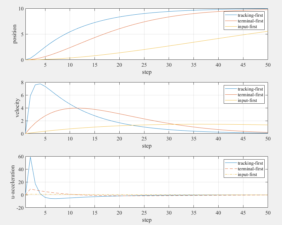
Analysis of Results

Performance Comparison

Based on the simulation results:

Tracking-First Strategy:

• Fastest convergence to reference values
• Higher control effort initially
• Excellent tracking throughout the trajectory
• Best for applications requiring tight tracking

Terminal-First Strategy:

• Balanced approach with moderate control effort
• Good final accuracy with flexible trajectory
• Smooth convergence without excessive overshoot
• Suitable for general regulation tasks

Input-First Strategy:

• Minimal control effort and energy consumption
• Slower convergence but very smooth response
• Conservative approach avoiding aggressive control
• Ideal for systems with actuator limitations

Design Trade-offs

Strategy	Convergence Speed	Control Effort	Energy Efficiency	Robustness
Tracking-first	Fast	High	Low	Medium
Terminal-first	Medium	Medium	Medium	High
Input-first	Slow	Low	High	High

Applications and Extensions

1. Multi-Reference Tracking

For time-varying references, the augmentation approach can be extended: $x^r_{k+1} = A_r x^r_k + B_r w_k$

Where $w_k$ represents reference dynamics inputs.

2. Integral Action

Add integral states to eliminate steady-state errors: $\xi_{k+1} = \xi_k + (x_k - x^r_k)$

3. Output Regulation

For output tracking problems: $y_k = C x_k \rightarrow y^r_k$

Modify the error definition to $e_k = y_k - y^r_k$.

4. Disturbance Rejection

Include disturbance models in the augmentation: $x_{k+1} = A x_k + B u_k + E d_k$

Design Guidelines

Weight Matrix Selection

For tight tracking:

• Use large $Q$ values
• Moderate $R$ values
• Accept higher control effort

For energy efficiency:

• Use large $R$ values
• Moderate $Q$ values
• Accept slower response

For balanced performance:

• Use moderate $Q$ and $R$ values
• Emphasize terminal accuracy with larger $S$

Practical Considerations

1. Actuator constraints: Choose $R$ to prevent saturation
2. Model uncertainties: Use conservative designs
3. Noise sensitivity: Balance performance vs. robustness
4. Computational limits: Consider real-time implementation requirements

Summary

The LQR set-point regulation framework provides:

• Systematic approach to reference tracking problems
• Optimal control subject to quadratic cost
• Flexible tuning through weight matrix design
• Practical implementation for real systems

The state augmentation technique transforms tracking problems into regulation problems, enabling the application of standard LQR theory to achieve optimal reference following.

References

1. Chris Mavrogiannis - LQR Tracking
2. Wang, T. (2023). 控制之美 (卷2). Tsinghua University Press.
3. Anderson, B. D. O., & Moore, J. B. (2007). Optimal Control: Linear Quadratic Methods. Dover Publications.
4. Lewis, F. L., Vrabie, D., & Syrmos, V. L. (2012). Optimal Control (3rd ed.). John Wiley & Sons.