Linear Quadratic Regulator for Discrete-Time Systems
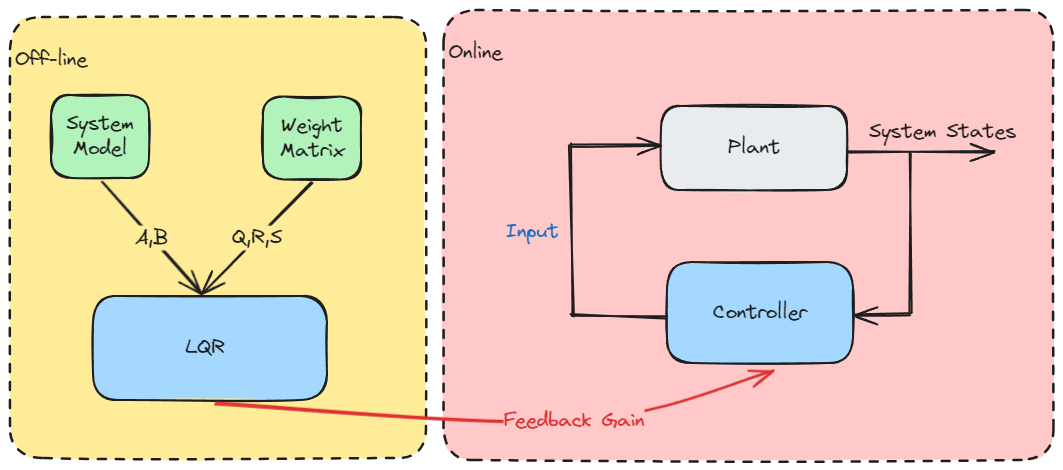
The Linear Quadratic Regulator (LQR) is one of the most important results in optimal control theory. This document presents the complete derivation and implementation of LQR for discrete-time linear systems using dynamic programming.
Problem Formulation
System Dynamics
Consider a discrete-time linear time-varying system:
Where:
- : state vector at time
- : control input at time
- : state transition matrix
- : input matrix
Quadratic Performance Function
The objective is to minimize the quadratic cost function:
Where:
The factor is included to simplify derivative calculations in the optimization process.
Weight Matrices
The weight matrices must satisfy certain definiteness conditions:
Terminal weight matrix:
State weight matrix:
Input weight matrix:
- : Positive semi-definite (allow zero eigenvalues)
- : Positive definite (all eigenvalues must be positive)
These conditions ensure the optimization problem is well-posed and has a unique solution.
Dynamic Programming Solution
Stage N: Terminal Stage ()
At the terminal stage, the cost-to-go is:
The optimal cost-to-go has the quadratic form:
Where we define: .
Stage N-1: One Step to Go ()
The cost-to-go from stage to is:
Substituting the system dynamics :
Optimization: Finding the Optimal Control
To find the optimal control, we take the derivative with respect to and set it to zero:
Derivative calculation:
For the first term, let :
For the second term:
Setting the derivative to zero:
Solving for the optimal control:
This gives us the feedback control law:
Where the feedback gain is:
Verification of Minimum
The second derivative confirms this is a minimum:
Since and , the Hessian is positive definite.
Cost-to-Go Matrix Update
Substituting the optimal control back into the cost function:
Where:
This is the discrete-time algebraic Riccati equation in recursive form.
General Recursive Solution
For Stage to
Optimal control:
Feedback gain:
Cost-to-go:
Riccati recursion:
Alternative Riccati Form
The Riccati equation can also be written as:
Algorithm Summary
Backward Pass (Offline Computation)
Initialize:
For :
- Compute feedback gain:
- Update Riccati matrix:
Forward Pass (Online Implementation)
Given: Initial state
For :
- Apply control:
- Update state:
Time-Invariant Case
For Linear Time-Invariant (LTI) systems where and are constant:
Steady-State Solution
As , the feedback gain converges to a constant:
The steady-state gain satisfies:
Where is the solution to the discrete-time algebraic Riccati equation (DARE):
Advantages of Steady-State Solution
- Computational efficiency: No need to solve Riccati recursion online
- Memory savings: Store only one gain matrix instead of sequence
- Stability guarantees: If is controllable and is observable
Implementation
MATLAB Implementation
function [F] = lqr_dp(A, B, Q, R, S)
% LQR solution using dynamic programming
% Inputs: A, B (system matrices), Q, R, S (weight matrices)
% Output: F (feedback gain)

    P0 = S;                    % Initialize P_[0]
    max_iter = 200;            % Maximum iterations
    tolerance = 1e-3;          % Convergence tolerance

    P_k_minus_1 = P0;
    F_prev = Inf;

    for k = 1:max_iter
        % Compute feedback gain
        F_current = (R + B' * P_k_minus_1 * B) \ (B' * P_k_minus_1 * A);

        % Update Riccati matrix
        P_k = (A - B * F_current)' * P_k_minus_1 * (A - B * F_current) + ...
              F_current' * R * F_current + Q;

        % Check convergence
        if max(abs(F_current - F_prev), [], 'all') < tolerance
            fprintf('Converged in %d iterations\n', k);
            F = F_current;
            return;
        end

        P_k_minus_1 = P_k;
        F_prev = F_current;
    end

    error('Maximum iterations exceeded');
end
Python Implementation
import numpy as np

def lqr_dp(A, B, Q, R, S):
    """
    LQR solution using dynamic programming
    """
    P0 = S                     # Initialize P_[0]
    max_iter = 200             # Maximum iterations
    tolerance = 1e-3           # Convergence tolerance

    P_k_minus_1 = P0
    F_prev = np.inf

    for k in range(max_iter):
        # Compute feedback gain
        F_current = np.linalg.solve(
            R + B.T @ P_k_minus_1 @ B,
            B.T @ P_k_minus_1 @ A
        )

        # Update Riccati matrix
        A_cl = A - B @ F_current
        P_k = A_cl.T @ P_k_minus_1 @ A_cl + F_current.T @ R @ F_current + Q

        # Check convergence
        if np.max(np.abs(F_current - F_prev)) < tolerance:
            print(f'Converged in {k+1} iterations')
            return F_current

        P_k_minus_1 = P_k
        F_prev = F_current

    raise ValueError('Maximum iterations exceeded')
Properties and Characteristics
1. Optimality
The LQR controller minimizes the quadratic cost function subject to the linear system dynamics.
2. Stability
For the infinite-horizon case, if is controllable, the closed-loop system is asymptotically stable.
3. Robustness
LQR controllers have excellent robustness properties:
- Gain margin: dB
- Phase margin:
4. Linear State Feedback
The optimal control law is a linear function of the current state, making it easy to implement.
Design Guidelines
Weight Matrix Selection
State weights ():
- Larger values → tighter regulation of corresponding states
- Zero diagonal elements → no penalty for deviations in those states
Input weights ():
- Larger values → more conservative control (smaller inputs)
- Smaller values → more aggressive control (larger inputs)
Terminal weights ():
- Often chosen as solution to infinite-horizon DARE
- Can be zero for finite-horizon problems
Tuning Process
- Start with identity matrices: ,
- Adjust relative weights based on performance requirements
- Use iterative design and simulation verification
- Consider physical constraints and actuator limitations
Extensions and Variations
1. LQR with Integral Action
Add integral states to eliminate steady-state error for step references.
2. LQG (Linear Quadratic Gaussian)
Combine LQR with Kalman filter for systems with noise and partial state measurements.
3. Robust LQR
Design controllers that maintain performance under model uncertainties.
4. Constrained LQR
Handle input and state constraints using model predictive control (MPC).
References
- Optimal Control by DR_CAN
- Wang, T. (2023). 控制之美 (卷2). Tsinghua University Press.
- Anderson, B. D. O., & Moore, J. B. (2007). Optimal Control: Linear Quadratic Methods. Dover Publications.
- Lewis, F. L., Vrabie, D., & Syrmos, V. L. (2012). Optimal Control (3rd ed.). John Wiley & Sons.
- Åström, K. J., & Murray, R. M. (2021). Feedback Systems: An Introduction for Scientists and Engineers (2nd ed.). Princeton University Press.